<?xml version="1.0" encoding="utf-8"?><feed xmlns="http://www.w3.org/2005/Atom" ><generator uri="https://jekyllrb.com/" version="3.10.0">Jekyll</generator><link href="https://rwharton.github.io/feed.xml" rel="self" type="application/atom+xml" /><link href="https://rwharton.github.io/" rel="alternate" type="text/html" /><updated>2024-09-07T21:39:52-07:00</updated><id>https://rwharton.github.io/feed.xml</id><title type="html">astronomy &amp;amp; software</title><subtitle>personal description</subtitle><author><name>Robert S. Wharton</name><email>rswharton95@gmail.com</email></author><entry><title type="html">Cold Streak Part 3: Markov Chain</title><link href="https://rwharton.github.io/posts/2024/09/07/streak-part3" rel="alternate" type="text/html" title="Cold Streak Part 3: Markov Chain" /><published>2024-09-07T00:00:00-07:00</published><updated>2024-09-07T00:00:00-07:00</updated><id>https://rwharton.github.io/posts/2024/09/07/win-streak-3</id><content type="html" xml:base="https://rwharton.github.io/posts/2024/09/07/streak-part3"><![CDATA[<p>This is Part 3 of a series exploring a particular probability 
problem encountered while watching my baseball team lose 
(they got <a href="https://www.mlb.com/standings/?date=2024-09-06">better</a>). 
In baseball terms, the question was <em>what is the maximum number 
of losses you expect a good team to have in any 20-game stretch 
during the season</em>. In mathematical terms, the problem can be 
stated as</p>

<blockquote>
  <p>Assume we have a binomial process that has two outcomes:
a win or a loss. Let \(p\) be the probability of a win,
so that \(1-p\) is the probability of a loss.  For a list
of \(N\) games, what is the probability that the highest
number of wins (or losses) in any \(M\) game window is
greater than or equal to \(k\).</p>
</blockquote>

<p>In <a href="/posts/2024/09/02/streak-part1">Part 1</a>, we were able 
to answer this question for particular \(N\), \(M\), \(k\), 
and \(p\) by simulating a large number of seasons and 
counting the max values.  It wasn’t an exact solution, 
but was pretty easy. In <a href="/posts/2024/09/05/streak-part2">Part 2</a>, 
we took a very different approach. We considered the very 
small case of \(N=5\) and \(M=3\) and wrote down all 
possible seasons. From this we could calculate the exact 
probabilites for all \(k\) values for any single game 
win probability \(p\). This is exactly what we want… 
except that this method quickly becomes impossibly 
complex.</p>

<p>In this Part 3, we will use what we learned in Part 2, 
but avoid enumerating all \(2^N\) possible season results. 
Instead, we will only keep track of the \(2^M\) possible 
results within a window. For \(N=162\) and \(M=20\), this 
means “only” having to enumerate \(\sim10^6\) states instead 
of the full \(\sim10^{49}\).  Progress!</p>

<h1 id="markov-process">Markov Process</h1>

<p>First, we will need to learn a little something about Markov 
processes. A <a href="https://en.wikipedia.org/wiki/Markov_chain">Markov process</a> 
is a certain type of random process that generates a series of events. 
In a simple case, let’s say we have two states: A and B. At each step, 
we can either transfer between the states or stay in the current state. 
A key property of Markov chains is that the transition probabilities 
depend <em>only on the current state</em>, so all that matters is if we are 
currently in state A or B.</p>

<p>To generate a list of events with the Markov process, we simply 
look at what state we are currently in, then draw the next state 
based on the transition probabilities. For our simple example, 
lets say that when we are in state A, we can switch to state B 
with probability \(p_{\rm AB} = 0.2\) or stay in state A with 
\(p_{\rm AA} = 0.8\).  When we are in state B, we can transfer to 
state A with probability \(p_{\rm BA} = 0.6\) or stay in state 
B with \(p_{\rm BB} = 0.4\).</p>

<p>If we start in state A, we can follow these rules to produce:</p>

\[\texttt{A A B B A A B A A A B}.\]

<h2 id="transition-matrix">Transition Matrix</h2>

<p>We can also write the probilities in the form of a transition matrix
(or <a href="https://en.wikipedia.org/wiki/Stochastic_matrix">stochastic matrix</a>).
Each element of the transition matrix, \(p_{ij}\), will give the probability 
of going from state \(i\) to state \(j\). If we call states A and B states 
0 and 1, we can write:</p>

\[\begin{pmatrix}
p_{00} &amp; p_{01} \\
p_{10} &amp; p_{11} \\
\end{pmatrix}
=
\begin{pmatrix}
p_{AA} &amp; p_{AB} \\
p_{BA} &amp; p_{BB} \\
\end{pmatrix}
= 
\begin{pmatrix}
0.8 &amp; 0.2 \\
0.6 &amp; 0.4 \\
\end{pmatrix}\]

<p>Though it may take a little getting used to, the transition matrix 
description of a Markov process will make our lives much easier when
we start calculating things.  Let’s start with an easy example.</p>

<p>If we start in State A, what are the probabilites that we are 
in each state after one step? Since it’s just one step, we know 
that the answers are just \(p_{AA}\) for state A and 
\(p_{AB}\) for state B.  But we can also calcualte this 
with the transition matrix:</p>

\[\begin{align}
\begin{pmatrix}
p_A &amp; p_B \\
\end{pmatrix}
&amp;=
\begin{pmatrix}
1 &amp; 0 \\
\end{pmatrix}

\begin{pmatrix}
p_{AA} &amp; p_{AB} \\
p_{BA} &amp; p_{BB} \\
\end{pmatrix}\\

&amp;= 
\begin{pmatrix}
1 \cdot p_{AA} + 0 \cdot p_{BA} &amp; 1\cdot p_{AB} + 0 \cdot p_{BB} \\
\end{pmatrix}\\

&amp;= 
\begin{pmatrix}
p_{AA} &amp; p_{AB} \\
\end{pmatrix} \\

&amp;= 
\begin{pmatrix}
0.8 &amp; 0.2 \\
\end{pmatrix}
\end{align}\]

<p>We can also do the same thing starting from state B:</p>

\[\begin{align}
\begin{pmatrix}
p_A &amp; p_B \\
\end{pmatrix}
&amp;=
\begin{pmatrix}
0 &amp; 1 \\
\end{pmatrix}

\begin{pmatrix}
p_{AA} &amp; p_{AB} \\
p_{BA} &amp; p_{BB} \\
\end{pmatrix}\\

&amp;= 
\begin{pmatrix}
0 \cdot p_{AA} + 1 \cdot p_{BA} &amp; 0\cdot p_{AB} + 1\cdot p_{BB} \\
\end{pmatrix}\\

&amp;= 
\begin{pmatrix}
p_{BA} &amp; p_{BB} \\
\end{pmatrix}\\

&amp;= 
\begin{pmatrix}
0.6 &amp; 0.4 \\
\end{pmatrix}
\end{align}\]

<p>where in each case we have specified the starting state 
via a <a href="https://en.wikipedia.org/wiki/Row_and_column_vectors">row vector</a>. 
I have gone through the operations to make clear how to multiply this 
with a matrix from the right. It’s a little different from what we 
typically see, but is just based on how the transition matrix is 
defined (you could make it a left transition matrix and operate on 
vectors by flipping rows and columns).</p>

<h2 id="many-steps">Many Steps</h2>

<p>One of the nice things about the transition matrix approach is that 
it allows us to calculate probabilities at step \(n\) fairly easily. 
Based on what we saw above for a single step, multiple steps can be 
calculated by repeated multiplications of the transition matrix. 
This is equivalent to a single multiplication of the transition 
matrix to the \(n\)-th power:</p>

\[P^n = 
\begin{pmatrix}
p_{AA} &amp; p_{AB} \\
p_{BA} &amp; p_{BB} \\
\end{pmatrix}^n \\\]

<p>We can now easily calculate this matrix for any \(n\) for the 
problem above.  We have</p>

\[\begin{align}
P^1 &amp;= 
\begin{pmatrix}
0.8  &amp;  0.2 \\
0.6  &amp;  0.4 \\
\end{pmatrix} \\

P^2 &amp;= 
\begin{pmatrix}
0.76  &amp;  0.24 \\
0.72  &amp;  0.28 \\
\end{pmatrix} \\

P^3 &amp;= 
\begin{pmatrix}
0.752  &amp;  0.248 \\
0.744  &amp;  0.256 \\
\end{pmatrix} \\

&amp;\vdots \\

P^{10} &amp;= 
\begin{pmatrix}
0.75  &amp;  0.25 \\
\end{pmatrix} \\

\end{align}\]

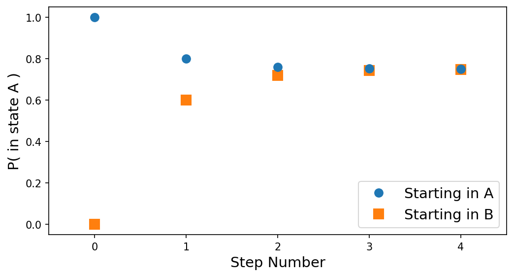
<p>where we see something interesting happening. As we get more 
and more steps, the rows of the matrix converge to the same 
values. This means the the probability of being in a given 
state is independent of the starting value.  We can see this 
beter in a plot:</p>

<p align="center">
  <img alt="Markov steps" src="/images/blog/bball-3/markov_fig1.png" width="500" />
  <br />
    Fig 1:  <em>Probability of being in state A after n steps assuming 
                we start in state A (blue circle) or state B (orange square)</em>
</p>

<p>This makes sense because the early steps will be affected 
by where we start, but eventually we get far enough away 
that we reach a steady state.</p>

<h2 id="absorbing-state">Absorbing State</h2>

<p>Now what would happen if we added a third state C, that 
would <em>only</em> transition to itself (\(p_{CC} = 1\))? Since 
it does not allow transitions to other states, the chain 
would get stuck in C. For this reason, these states are 
called “absorbing states”.</p>

<p>Let’s modify our example above to include an absorbing 
state. Consider the transition matrix:</p>

\[P = 
\begin{pmatrix}
0.7  &amp;  0.2  &amp; 0.1 \\
0.5  &amp;  0.3  &amp; 0.2 \\
0    &amp;   0   &amp; 1 \\
\end{pmatrix}\]

<p>which means A goes to \((A, B, C)\) with probability 
\((0.7, 0.2, 0.1)\), B goes to the same with 
probability \((0.5, 0.3, 0.2)\) and C only goes 
to C.</p>

<p>Since all states can go to C, but once there cannot leave, 
then eventually everything will go to state C.  We can see 
this by calculating the result after, say, 10 steps:</p>

\[P^{10} \approx  
\begin{pmatrix}
0.20  &amp; 0.07  &amp;  0.73  \\
0.17  &amp; 0.06  &amp;  0.77  \\
0     &amp;  0    &amp;  1     \\
\end{pmatrix}\]

<p>and after 20:</p>

\[P^{20} \approx  
\begin{pmatrix}
0.05  &amp; 0.02  &amp;  0.93  \\
0.04  &amp; 0.01  &amp;  0.94  \\
0     &amp;  0    &amp;  1     \\
\end{pmatrix}\]

<p>where each row indicates the probability of being 
in states \((A, B, C)\) for starting state \(A\) (top row), 
\(B\) (middle row), and \(C\) (bottom row).</p>

<p>Absorbing states are useful for indicating a stopping condition, 
since once they reach that state, nothing changes. This is 
exactly what we will use an absorbing state for.</p>

<h1 id="back-to-baseball">Back to Baseball</h1>

<p>Now that we have a bit of background on Markov processes, let’s see 
if we can apply it to the problem at hand.  Once again, our problem 
is</p>

<blockquote>
  <p>Assume we have a binomial process that has two outcomes:
a win or a loss. Let \(p\) be the probability of a win,
so that \(1-p\) is the probability of a loss.  For a list
of \(N\) games, what is the probability that the highest
number of wins (or losses) in any \(M\) game window is
greater than or equal to \(k\).</p>
</blockquote>

<p>So we want to keep track of the number of wins (or losses) 
in a running window of \(M\) games. But that depends on the 
current game <strong>and</strong> the \(M-1\) previous games. The <strong>one</strong> 
rule we learned about a Markov process is that it is memoryless 
and can <strong>only</strong> depend on the current state. That is true, 
but we can be tricky about what we call a state.</p>

<h2 id="picking-a-state">Picking A State</h2>

<p>One potential option is to enumerate every single possible 
combination of \(1\)s and \(0\)s in an \(M\) game window. 
From <a href="/posts/2024/09/05/streak-part2">Part 2</a>, we know that 
there are \(2^M\) ways to make a length \(M\) string of 
\(0\)s and \(1\)s. That could potentially get pretty 
unwieldy for large \(M\), but it sure beats enumerating 
every result in the season like we did in Part 2. But 
does it satisfy the Markov condition?</p>

<p>A Markov process has to be memoryless, which means that the 
transition properties can only depend on the current state. 
Let’s say that we have \(M=5\), then one of our states will 
be</p>

\[s_i = 01101.\]

<p>The next possible state is just the string of 5 bits you 
get by shifting the window over one game. So for this 
state, the possible next states are:</p>

\[s_{i+1} = 
\begin{cases}
11010, &amp; \text{if next value is 0} \\
11011, &amp; \text{if next value is 1}
\end{cases}\]

<p>because by moving our window one game over, we have 
lost the trailing \(0\) and picked up either a \(0\) 
or a \(1\).</p>

<p>We can also very easily calculate the transition probabilities 
are because it is simply the probability of getting a one, \(p\), 
or getting a zero \(1-p\). Thus the transition probabilities 
<em>only</em> depend on the current state, which satisfies the Markov 
condition.</p>

<h2 id="transitions">Transitions</h2>

<p>Since we are enumerating all \(2^M\) possible combinations 
for the contents of our length \(M\) window, we are going to 
have to be very careful about bookkeeping. If \(M=20\), 
we will have \(2^{20} \approx 10^6\) possible states. That’s 
too many to go through and identify by hand. Fortunately, we
can use a clever trick we found in Part 2.</p>

<p>A simple way to enumerate all the \(2^M\) strings of zeros 
and ones is to simply count to \(2^M\) in binary (pre-pending 
zeros as necessary).  So for \(M=5\) we would have</p>

\[\begin{align}
0 &amp;= 00000 \\
1 &amp;= 00001 \\
2 &amp;= 00010 \\
\vdots &amp; \\
29 &amp;= 11101 \\
30 &amp;= 11110 \\
31 &amp;= 11111 
\end{align}\]

<p>This means that we could keep track of each state by recording 
the base-10 number the corresponds to the binary string. This 
makes things much easier. Now, instead of storing, for example,
a 15 game string of wins and losses as</p>

\[s_i = 111101010110111\]

<p>we can instead just store the number</p>

\[s_i = 31415\]

<p>Not bad!</p>

<p>But is there any way to figure what states this 
can transition to? Consider the state:</p>

\[s_i = 11101.\]

<p>It can transition to the following states:</p>

\[s_{i+1} = 
\begin{cases}
11010, &amp; \text{if next value is 0} \\
11011, &amp; \text{if next value is 1}
\end{cases}\]

<p>We described this in terms of shifting the \(M\) game 
window, but if we take the binary represenation seriously,
then shifting one spot to the left is the same as multiplication 
by 2. As our window moves one spot right, all the numbers move 
one spot to the left, meaning one higher power of two. Now, 
there is a little bit of a catch because we are dropping the 
previously leftmost value. But that’s not a problem because 
we can just calculate the number 
<a href="https://en.wikipedia.org/wiki/Modulo">modulo</a> 
\(2^M\). The modulo is simply the remainder after dividing 
by \(2^M\). Since all of our states are by construction 
less than \(2^M\), this will give us what we want.</p>

<p>Let’s give it a try.  The state \(s_i = 11101\) is the 
binary representation of the (base-10) number 29. So:</p>

\[(29 \times 2) \mathbin{\rm mod} 2^5 = 58 \mathbin{\rm mod} 32 = 26\]

<p>and 26 in binary is \(11010\), which is indeed one of 
the answers that we were looking for.  Since we are mutliplying 
by 2 and taking the modulo with respect to another even number, 
the result here will always be even. But the other valid state 
is exactly the same except the last bit is a 1.  That means 
you just have to add one.</p>

<p>This means that for a given state \(s_i\) in base-10 representation,
we can calculate the valid transitions as:</p>

\[s_{i+1} = 
\begin{cases}
2 s_i \mathbin{\rm mod} 2^M, &amp; \text{newest val a 0} \\
2 s_i \mathbin{\rm mod} 2^M + 1, &amp; \text{newest val a 1}
\end{cases}\]

<p>and the probability of making these transitions is just 
\(p\) if the newest value is a one and \(1-p\) if the 
newest value is a zero.</p>

<h2 id="stopping-condition">Stopping Condition</h2>

<p>Now that we have a neat way to represent our states, we should 
really go back to the problem. What is it we are trying to do 
again? We want to find the probability of getting at least \(k\) 
wins (or losses) in any \(M\) length stretch of games in an 
\(N\) length season. Therefore once we hit a state with \(k\) 
or more wins, we can stop, since our season has already met 
the goal. This sounds like the perfect case for an absorbing 
state!</p>

<p>For any value of \(k\), we will have some states that have 
less than \(k\) wins and others that will have at least 
\(k\) wins. The latter states are really just one state 
then.  That is, they are the state where we have met our 
goal. If we call the states with less than \(k\) wins 
“valid” states then the total number of states we need 
to consider are \(n_{\rm valid} + 1\). This number will 
be less than \(2^M\), but will still be roughly the same 
order of magnitude.</p>

<h2 id="building-the-transition-matrix">Building the Transition Matrix</h2>

<p>To build our transition matrix, we need to calculate \(p_{ij}\) 
between all possible states. But as we have seen above, any given 
state can transition to 2 other states with probability \(p\) if 
it ends in \(1\) or \((1-p)\) if it ends in 0.  That means that 
most of our transition matrix will have rows that are mostly zero, 
but with two nonzero entries.  The final absorbing state, however,
will be all zeros except for a single entry of \(1\).</p>

<p>Previously we showed that any given state could be represented 
as a binary string which could then be turned into a base-10 
number. We could then just index each state by this base-10 number, 
which would be pretty easy.  However, some of these states will 
have have at least \(k\) wins and so would be absorbing states. 
We need to just have one absorbing state, so we will have to map 
all of these to the same index. This means we lose the easy indexing 
of states and are required to do one extra step where we map 
the base-10 number to the index value.</p>

<p>OK, so let’s try building the case where \(N=5\), \(M=3\), and 
we want \(k \geq 2\). For simplicity, let’s set \(p=0.5\). The 
valid states will have no more than 1 win. For \(M=3\), there 
are only 4 valid states:</p>

\[\begin{align}
0 &amp;: 000 \\
1 &amp;: 001 \\
2 &amp;: 010 \\
4 &amp;: 100 \\
\end{align}\]

<p>since any other state would have at least 2 ones. We then add 
one absorbing state to get a total of 5 possible states for this 
process.</p>

\[P = 
\begin{pmatrix}
0.5   &amp;  0.5 &amp;   0  &amp;    0  &amp;    0  \\   
 0    &amp;   0  &amp;  0.5 &amp;    0  &amp;   0.5 \\
 0    &amp;   0  &amp;   0  &amp;   0.5 &amp;   0.5 \\
0.5   &amp;  0.5 &amp;   0  &amp;    0  &amp;    0  \\
 0    &amp;   0  &amp;   0  &amp;    0  &amp;    1  \\ 
\end{pmatrix}\]

<p>The first row is for \(000\), which can only transition 
to \(000\) (if the next val is a 0) or \(001\) if the next 
value is 1.  The second row is for \(001\) which can only 
go \(010\) or \(011\), which has two wins and thus goes 
to the absorbing state.  The third row is for \(010\), 
which can go to \(100\) or \(101\), which has two wins 
and thus also goes to the absorbing state.  The fourth 
row is for \(100\) which can go to \(000\) or \(001\).
The fifth row is the absorbing state, which can only go 
to itself with probability 1.</p>

<h2 id="calculating-the-probability">Calculating the Probability</h2>

<p>Now that we have our transition matrix, we know how to 
calculate the probability that our system is in a given 
state after \(n\) steps.  That would just be \(P^n\). 
But the way we have defined our states and the way we 
constructed our transition matrix means that we do not 
account for the starting point. We <em>start</em> with a state 
of \(M\) games. That means two things.  First, we only 
need to propagate our system through \(N-M\) steps.
Second, it means that we need to calculate the probability 
of starting in each given state.</p>

<p>Following with our simple example, if we want to calculate 
the probability that we start with state \(000\) and it 
ends up with \(k\geq2\), then we would do</p>

\[P(s_0 = 000, k\geq2) = P(s_0 = 000) \cdot P(k\geq2 | s_0 = 000)\]

<p>In Part 2, we showed that the probability of getting \(n_0\)
zeros and \(n_1\) ones in a string of length \(M\) is</p>

\[P(s_i) = p^{n_1} (1-p)^{n_0}.\]

<p>For the absorbing state, its a little bit different because 
it encompasses all states with at least \(k\) ones. But for 
that we can use the
<a href="https://en.wikipedia.org/wiki/Binomial_distribution">binomial distribution</a>:</p>

\[P(s_4) = P(\geq k) = \sum_{s=k}^{M} {M\choose s} p^s (1-p)^{M-s}.\]

<p>The probability of getting \(k\geq 2\) at least once 
for each starting state can be read off from the final 
\(N-M\) step transition matrix, \(P^{N-M}\), in the last 
column in the row corresponding to the initial state.</p>

<p>For the transition matrix above with \(N=5\), \(M=2\), and 
\(p=0.5\), we have</p>

\[P^{5-3} = P^2 = 
\begin{pmatrix}
0.25  &amp;  0.25  &amp; 0.25  &amp;  0    &amp; 0.25 \\ 
 0    &amp;   0    &amp;  0    &amp; 0.25  &amp; 0.75 \\ 
0.25  &amp;  0.25  &amp;  0    &amp;  0    &amp; 0.50 \\ 
0.25  &amp;  0.25  &amp; 0.25  &amp; 0     &amp; 0.25 \\ 
 0    &amp;   0    &amp;  0    &amp; 0     &amp; 1 \\ 
\end{pmatrix}\]

<p>So the final answer will be the sum over all states 
of the probability of starting in the state times 
the probability of that state ending in the absorbing 
state. That is:</p>

\[P(k\geq 2) = \sum_{i=0}^{4} P(s_i) P^2_{i4}\]

<p>We would then get:</p>

\[\begin{align}
P(k\geq 2) = &amp; \left[ (0.5^3) (0.25) \right]_{000} \\ 
             &amp;  + \left[ (0.5^2 \cdot 0.5) (0.75) \right]_{001} \\
             &amp; + \left[ (0.5^2 \cdot 0.5) (0.50) \right]_{010}  \\
             &amp;  + \left[ (0.5^2 \cdot 0.5) (0.25) \right]_{100}  \\
             &amp; + \left[ (3 \cdot 0.5^2 \cdot 0.5 + 0.5^3) (1) \right]_{\rm absorb} \\
           = &amp; \frac{23}{32}
\end{align}\]

<p>In Part 2 we found that the probability of getting exactly 2 wins 
was \(15/32\) and the probability of getting exactly 3 wins was 
\(1/4\).  Summing those gives a probability for \(k\geq 2\) of 
\(23/32\), which is exactly what we have here.  That’s good!</p>

<h1 id="what-have-we-done">What Have We Done?</h1>

<p>This part ended up being a bit longer than I expected, so maybe 
it is useful to stop here and take stock of where we are. We 
developed a way to calculate the answer to our question using 
methods for Markov processes. For arbitrary values of \(N\), 
\(M\), \(k\), and \(p\) we can in principle enumerate the 
states, construct a transition matrix, and then finally calculate 
the total probability of getting at least one \(M\) game window 
with \(k\) or more wins.</p>

<p>This is an important achievement over our initial simulations 
because (up to numerical error), we know that the result we 
get will be exactly correct. However, this is still just a 
calculation, we have not found an equation to just plug in 
our parameters and get an answer. Instead we just have a 
method of getting the answer without any of the insight 
of an equation.</p>

<p>There is one big remaining problem, though. Our test case 
was the very small example we were able to previously work 
out by hand. Our calculation here requires a transition 
matrix that will be roughly \(2^M \times 2^M\) in size and 
we need to then calculate the \(N-M\)-th power of that matrix.
At some point we are going to run into some performance issues.
But we’ll deal with that next time!</p>

<!---
<p align="center">
  <img alt="phriendship" src="/images/blog/bball-3/alvarado.png" width="500">
  <br>
    <em>Phillies pitcher Jose Alvarado with a friendship necklace (not a Markov Chain)</em>
</p>
--->]]></content><author><name>Robert S. Wharton</name><email>rswharton95@gmail.com</email></author><category term="Baseball" /><category term="Markov" /><summary type="html"><![CDATA[This is Part 3 of a series exploring a particular probability problem encountered while watching my baseball team lose (they got better). In baseball terms, the question was what is the maximum number of losses you expect a good team to have in any 20-game stretch during the season. In mathematical terms, the problem can be stated as]]></summary></entry><entry><title type="html">Cold Streak Part 2: Counting</title><link href="https://rwharton.github.io/posts/2024/09/05/streak-part2" rel="alternate" type="text/html" title="Cold Streak Part 2: Counting" /><published>2024-09-05T00:00:00-07:00</published><updated>2024-09-05T00:00:00-07:00</updated><id>https://rwharton.github.io/posts/2024/09/05/win-streak-2</id><content type="html" xml:base="https://rwharton.github.io/posts/2024/09/05/streak-part2"><![CDATA[<p>This is Part 2 in our ongoing exploration of the important 
question <em>how bad can a good baseball team be?</em>
In <a href="/posts/2024/09/02/streak-part1">Part 1</a>, we solved
the problem in a quick, easy, but approximate way 
by running a bunch of simulations. Here we will 
consider a slow, painful, but exact way of solving 
our problem by enumerating states.</p>

<h1 id="the-problem">The Problem</h1>

<p>Although I will probably keep using the terminology of the 
baseball season example that motivated this problem, we are 
mostly interested in a mathematical problem and it is important 
to state it in such terms.  From Part 1, we will state our 
problem this way:</p>

<blockquote>
  <p>Assume we have a binomial process that has two outcomes: 
a win or a loss. Let \(p\) be the probability of a win, 
so that \(1-p\) is the probability of a loss.  For a list 
of \(N\) games, what is the probability that the highest 
number of wins (or losses) in any \(M\) game window is 
greater than or equal to \(k\).</p>
</blockquote>

<p>Our goal is to calculate this probability for any given 
values of \(p\), \(N\), and \(M\).</p>

<h1 id="starting-small">Starting Small</h1>

<p>To get our bearings, we will spend this post working through a 
small example where we can actually enumerate all the possible 
win loss combinations. Consider a season of \(N=5\) games where 
we will consider windows of size \(M=3\). A 5 game season could 
then look like this:</p>

\[S = \texttt{WWLWL}\]

<p>where the Ws are wins and the Ls are losses. It will be more 
convenient later on to represent the wins with a 1 and losses 
with a 0 so that the same season would look like this:</p>

\[S = 11010\]

<p>For a \(N=5\) game season, we can form three \(M=3\) game 
windows and count the wins:</p>

\[\begin{align}
 W_1 = &amp;110\hphantom{10}           ~\rightarrow~\textrm{2 wins} \\
 W_2 = &amp;\hphantom{1}101\hphantom{0}~\rightarrow~\textrm{2 wins}\\
 W_3 = &amp;\hphantom{10}010           ~\rightarrow~\textrm{1 win} \\
\end{align}\]

<p>so the maximum wins in a 3-game window for this season is 2.</p>

<p>From this simple example, we can already learn some things about 
the more general case.  Since each game has exactly two possible 
outcomes (0 or 1), there will \(2^N\) possible ways to generate 
a list of \(N\) 0s and 1s.  That means that there are \(2^N\) 
possible seasons. We can also see that for an \(N\) game season,
there will be \(N-M+1\) possible windows of length \(M\).</p>

<h1 id="representing-seasons">Representing Seasons</h1>

<p>Coming back to the \(N=5\) case, we see that there are only 
\(2^5=32\) possible seasons (which is a <strong>lot</strong> easier to 
deal with than the \(2^{162} \sim 10^{49}\) possible 
combinations for a full 162-game season). This means that 
we can very easily just write down all of the possible 
\(N=5\) game seasons. An easy way to do this is to note that 
any string of 0s and 1s is just a binary number. Just like 
we can write the base-10 representation of a number as</p>

\[42 = 4 \times 10^1 + 2 \times 10^0\]

<p>we can write its binary (base-2) representation as</p>

\[101010 = 1 \times 2^5 + 0 \times 2^4 + 1 \times 2^3 
            + 0 \times 2^2 + 1 \times 2^1 + 0 \times 2^0\]

<p>So enumerating all \(N=5\) length lists of 0s and 1s is 
equivalent to writing down the binary representation of 
the numbers 0 (00000) to 31 (11111).  This is a neat little 
trick that we will be taking advantage of later.</p>

<h1 id="enumerating-seasons">Enumerating Seasons</h1>

<p>We can now enumerate all possible season results 
(i.e., all ways to write down a combination of 
5 ones and zeros). The 32 possible seasons for 
\(N=5\) are thus:</p>

\[\begin{array}{c}
00000  &amp;   00001   &amp;   00010   &amp;   00011  \\[5pt]

00100  &amp;   00101   &amp;   00110   &amp;   00111  \\[5pt]   

01000  &amp;   01001   &amp;   01010   &amp;   01011  \\[5pt]

01100  &amp;   01101   &amp;   01110   &amp;   01111  \\[5pt]

10000  &amp;   10001   &amp;   10010   &amp;   10011  \\[5pt]

10100  &amp;   10101   &amp;   10110   &amp;   10111  \\[5pt]

11000  &amp;   11001   &amp;   11010   &amp;   11011  \\[5pt]

11100  &amp;   11101   &amp;   11110   &amp;   11111  \\[5pt]    
\end{array}\]

<p>Now we can just step through each of the three \(M=3\) 
length windows for each season and find the maximum 
number of 1s that occur.  Since we only have 32 different 
seasons, we can just count this manually:</p>

\[\begin{array}{c|c|c|c}
00000  &amp;   00001   &amp;   00010   &amp;   00011  \\
 0    &amp;     1     &amp;     1     &amp;     2    \\[5pt]
\hline

00100  &amp;   00101   &amp;   00110   &amp;   00111  \\
  1    &amp;     2     &amp;     2     &amp;     3    \\[5pt]
\hline

01000  &amp;   01001   &amp;   01010   &amp;   01011  \\
  1    &amp;     1     &amp;     2     &amp;     2    \\[5pt]
\hline

01100  &amp;   01101   &amp;   01110   &amp;   01111  \\
  2    &amp;     2     &amp;     3     &amp;     3    \\[5pt]
\hline

10000  &amp;   10001   &amp;   10010   &amp;   10011  \\
  1    &amp;     1     &amp;     1     &amp;     2    \\[5pt]
\hline

10100  &amp;   10101   &amp;   10110   &amp;   10111  \\
  2    &amp;     2     &amp;     2     &amp;     3    \\[5pt]
\hline

11000  &amp;   11001   &amp;   11010   &amp;   11011  \\
  2    &amp;     2     &amp;     2     &amp;     2    \\[5pt]
\hline

11100  &amp;   11101   &amp;   11110   &amp;   11111  \\
  3    &amp;     3     &amp;     3     &amp;     3    \\
\end{array}\]

<p>Since our window size is 3, the only allowed 
max values are 0, 1, 2, and 3 (that is, you can’t 
win more than 3 times in 3 games, no matter how hard 
you try).  Let’s count how many of the season have 
each of thse \(k\) values:</p>

\[\begin{align}
 n(k=0) &amp;= 1 \\ 
 n(k=1) &amp;= 8 \\ 
 n(k=2) &amp;= 15 \\ 
 n(k=3) &amp;= 8 \\ 
\end{align}\]

<h1 id="probability-special-case">Probability (Special Case)</h1>

<p>Now let’s consider a special case where the probability 
of a win is 0.5.  That means that we are equally likely 
to draw a 1 or a 0. It also means that all seasons are 
equally likely, with</p>

\[p_{S} = p^N = (1/2)^N = 2^{-N}\]

<p>which for \(N=5\) means \(p_{S} = 1/32\) for all 
seasons.  Since all season have equal probability 
<em>in this special case</em>, we can calculate the probability 
of getting specific \(k\) values by counting the number 
of seasons with those \(k\) values and dividing by the 
total number of all seasons, so</p>

\[p(k) = \frac{n(k)}{2^N}\]

<p>and thus</p>

\[\begin{align}
 p(k=0) &amp;= 1/32 \\ 
 p(k=1) &amp;= 8/32 = 1/4\\ 
 p(k=2) &amp;= 15/32 \\ 
 p(k=3) &amp;= 8/32 = 1/4 \\ 
\end{align}\]

<p>So just by counting we could calculate the probability 
for each \(k\) value for \(N=5\), \(M=3\), and \(p=0.5\).
But what about arbitrary win probabilities, \(p\)?</p>

<h1 id="probability-general-case">Probability (General Case)</h1>

<p>The \(p=0.5\) case was a simple matter of counting, but
what about general \(p\)?  Well, it’s a tiny bit more 
complicated, but we can do that as well. The difference 
will be that the seasons are no longer equally likely. 
To see this consider \(p=0.99\) where you have a 99% 
chance of winning any game.  Then surely winning all 
five and losing all 5 have very different chances of 
happening.</p>

<p>Let’s now calculate the probability of a particular 
season happening. Since the probability of getting a 
1 (a win) is \(p_1  = p\), then the probability of getting 
a 0 (a loss) is \(p_0 = 1 - p\).  Since the games are 
independent events, the probability of the season 
is just the product of the probabilities of the individual 
games.</p>

<p>So the probability of getting season \(01101\) is</p>

\[\begin{align}
P(01101) &amp;= p_0 \cdot p_1 \cdot p_1 \cdot p_0 \cdot p_1 \\
          &amp;= p_1^3 \cdot p_0^2 \\
          &amp;= p^3 \,(1-p)^2
\end{align}\]

<p>From this example, we see that the probability of any given 
season is determined just by the total number of wins.  If 
we call the number of wins \(s\), then the number of losses 
is \(N-s\) and the probability of that season is</p>

\[P(s) = p^s \, (1-p)^{N-s}\]

<p>To calculate the probability of the \(k\) values, we can 
utilize the enumeration table above, but we can’t use the 
total counts for each \(k\) like we did before.  This is 
because the probability of each season is no longer the same 
and so not all \(k=2\) (for example) are equally likely.</p>

<p>Instead, we will use the 
<a href="https://en.wikipedia.org/wiki/Law_of_total_probability">Law of Total Probability</a> 
and write:</p>

\[P(k) = \sum_{i=0}^{2^N} P(k | S_i) P(S_i)\]

<p>where the term \(P(k | S_i)\) is a conditional probability that 
means the probability of getting \(k\) assuming you are in 
season \(S_i\).  So in words this statement means that the 
probability of getting max counts \(k\) is equal to the sum 
(over all possible seasons) of the probability of getting \(k\) 
in seasons \(S_i\) times the probability of getting season 
\(S_i\).</p>

<p>We know how to calculate \(P(S_i)\), but what about the other 
term, \(P(k | S_i)\)? With our lookup table, this is simple 
because it will 1 if \(k=k_i\) and zero otherwise.  For 
the season \(01101\), we have a \(k=2\), so</p>

\[P(k | 01101) = 
\begin{cases}
1, &amp; k=2 \\
0, &amp; \text{otherwise}
\end{cases}\]

<p>Now we have enough information to calculate the exact probabilites 
for each \(k\) value for any win probability \(p\). We just generate 
all the valid seasons, count the \(k\) value for each season, and 
compute the probability for the season based on \(p\).  We then 
use the law of total probability to sum everything up.  The results 
are shown below and compared to the results from simulations.</p>

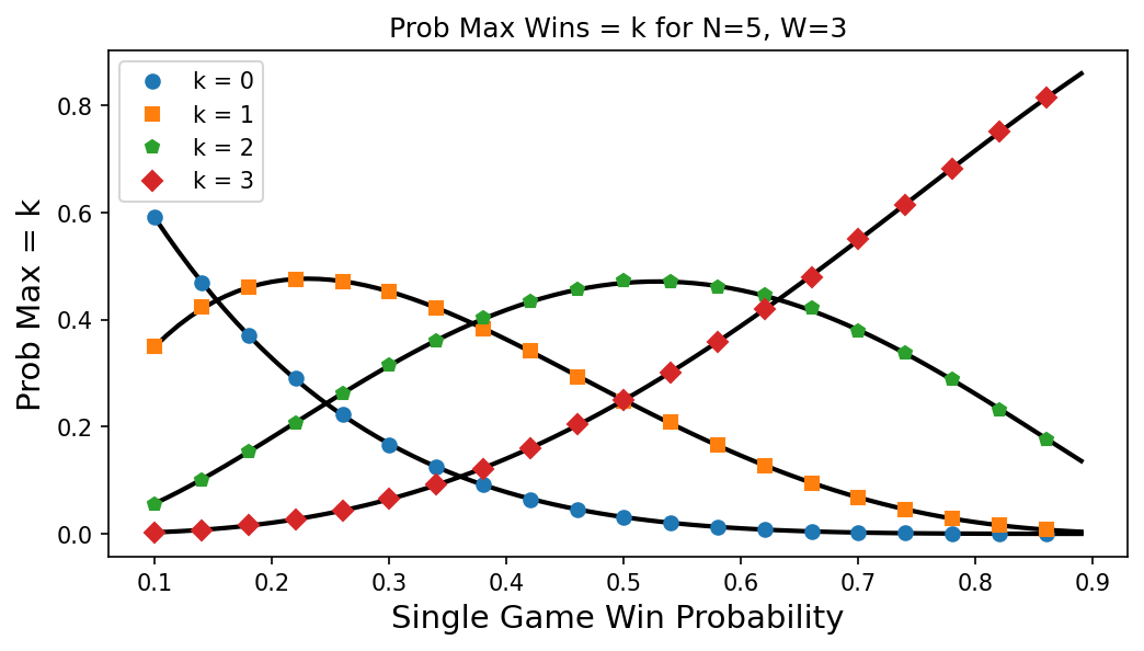
<p align="center">
  <img alt="Sim" src="/images/blog/bball-2/p2_fig1.png" width="500" />
  <br />
    Fig 1:  <em>The curves show the exact probabilities calculated 
                as described.  The symbols show the probabilities 
                estimated by the simulations we ran in Part 1.</em>
</p>

<p>Our calculated probabilities line up really well with the simulation
results.  The curves also behave as we would expect for varying values 
of individual game win probability \(p\). When \(p\) is very small, 
the lower \(k\) values dominate and then as \(p\) gets close to one, 
the higher values dominate. Also note that at \(p=0.5\), the probability 
of getting \(k=1\) is the same as \(k=3\), which we had found in our 
special case.</p>

<h1 id="conclusions">Conclusions</h1>

<p>The purpose of this post was mostly to define some of our terms 
and hopefully gain some intuition for this problem. Enumerating 
all of the seasons in a small \(N\) case is useful for getting a 
sense of the problem but is a <strong>highly</strong> impractical means for 
getting an answer.  For \(N=5\), we could pretty easily work 
with the 32 different seasons, but it was still tedious.  As 
\(N\) gets bigger, this method not only becomes a pain, it also 
becomes impossible.  You simply cannot list \(2^{162}\) different 
outcomes for a standard baseball regular season.</p>

<p>In Part 3, we’ll try a method that only requires us to keep track 
of the games in the running window of length \(M\).  That’s something 
thats more practical.  Well… maybe.</p>

<!---
<p align="center">
  <img alt="Harper Count" src="/images/blog/bball-2/harper3.jpg" width="500">
  <br>
    <em>Bryce Harper counting to three (Image Credit: Gregory Bull / AP)</em>
</p>
--->]]></content><author><name>Robert S. Wharton</name><email>rswharton95@gmail.com</email></author><category term="Baseball" /><category term="Counting" /><summary type="html"><![CDATA[This is Part 2 in our ongoing exploration of the important question how bad can a good baseball team be? In Part 1, we solved the problem in a quick, easy, but approximate way by running a bunch of simulations. Here we will consider a slow, painful, but exact way of solving our problem by enumerating states.]]></summary></entry><entry><title type="html">Quantifying A Cold Streak</title><link href="https://rwharton.github.io/posts/2024/09/02/streak-part1" rel="alternate" type="text/html" title="Quantifying A Cold Streak" /><published>2024-09-02T00:00:00-07:00</published><updated>2024-09-02T00:00:00-07:00</updated><id>https://rwharton.github.io/posts/2024/09/02/win-streak-1</id><content type="html" xml:base="https://rwharton.github.io/posts/2024/09/02/streak-part1"><![CDATA[<p>There’s an old Mitch Hedberg joke that goes “rice is great if you’re 
really hungry and want to eat two thousand of something.”  Baseball 
is kind of like that.  You have 162 games in the regular season where 
nine batters will get 3-5 chances to hit each game per team. The chance 
of getting a hit ranges from about 10% (not very good player) to about 
30% (very good player) for each attempt. Over the course of the long 
season, a player can string together a series of hits (hot streak) or 
a series of outs (cold streak).  These streaks could be due to something 
the player is doing (with the intrinsic probability of a hit changing), 
but can often be explained by statistical variance (with a fixed probability).</p>

<p>The same thing can happen when we consider the team as a whole. A team that 
wins 100 out its 162 games is very good (usually enough to win the division). 
However, this is only a winning percentage of about 62%.  Better than flipping 
a coin, but not by a whole lot. So again, just by statistical chance, you could 
get hot streaks (win a bunch) or cold streaks (lose a bunch). But it is also 
possible that the team is just getting better or worse. Is there a way to 
tell the difference?  Can we quantify when to panic?</p>

<h1 id="motivation">Motivation</h1>

<p>This exercise is mostly motivated by watching the ups and then 
sustained downs of my team, the Philadelphia Phillies.  After 
getting out to a really hot start, the team started losing a lot 
more often in July and into August. Despite continuing to have 
one of (if not the) best record in baseball, fans started to panic. 
Sensing an opportunity to smugly explain this away as statistical 
variance, I took a look at the numbers<sup id="fnref:1" role="doc-noteref"><a href="#fn:1" class="footnote" rel="footnote">1</a></sup>.</p>

<p>Grabbing the results for the 112 games at that point from 
<a href="https://www.baseball-reference.com">baseball-reference.com</a>, 
we can get a sense for how things changed over the course of 
the season (to that point). First we can plot the cumulative 
win fraction for the season.  That is, 
for each game, we add up all the wins to that point and divide by the 
total number of games to that point.  This will vary a lot early on 
because each game counts for more of the average, but will eventually 
steady out as each game is relatively less and less important.  The 
results are shown in the next plot:</p>

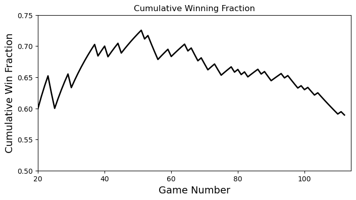
<p align="center">
  <img alt="Cumulative Win Rate" src="/images/blog/bball/tot_rate_fig.png" width="500" />
  <br />
    Fig 1:  <em>Cumulative win rate for the season</em>
</p>

<p>which tracks with experience. To get a sense for how good that peak is, 
note that only 15 teams have finished a season with a winning 
percentage above 70% (see <a href="https://en.wikipedia.org/wiki/List_of_best_Major_League_Baseball_season_win%E2%80%93loss_records">here</a>).</p>

<p>But if we are looking for ups and downs, maybe it is better to 
consider stretches of games.  For example, we can check the 
win fraction for a rolling 20-game window.  That is, we look 
at the last 20 games and calculate the fraction of games that 
were wins.  We then go to the next game and do the same.  This 
means that at each step we are adding the most recent game and 
removing the last game in the window.  The results are shown in 
the following plot:</p>

<p align="center">
  <img alt="Window Wins" src="/images/blog/bball/roll_20_fig.png" width="500" />
  <br />
    Fig 2:  <em>Winning Rate in a rolling 20 game window</em>
</p>

<p>This plot certainly tracks with how the season has felt.  The team 
got off to a very hot start, then eventually started cooling off 
and losing more and more games.</p>

<p>Now we can finally get to the point: the highest win rate for a 
20 game stretch this season is 0.85 and the lowest is 0.30.  Are 
these consistent with a good team that will win 95-100 games?</p>

<h1 id="the-problem">The Problem</h1>

<p>Let’s try to state the problem mathematically.  Assume we have 
a binomial process that has two outcomes: a win or a loss. 
Let \(p\) be the probability of a win, so that \(1-p\) is the 
probability of a loss.  For a list of \(N\) games, what is 
the probability that the highest number of wins (or losses) 
in any \(M\) game window is greater than or equal to \(k\). 
For Figure 2, we have \(N=112\) and \(M=20\).  The max number 
of observed wins in a window is 17 and the max number of observed 
losses in a window is 14. We want to determine if these are 
statistically significant deviations for some given winning 
probability of \(p\).</p>

<p>Note that rolling \(M\) game window makes things a little 
tricky. If we had just said <em>What is the probability that 
we get k or more wins in a list of M games?</em>, then the 
solution would be given by the 
<a href="https://en.wikipedia.org/wiki/Binomial_distribution">binomial distribution</a>, 
which we could easily calculate. If we were considering independent 
groups of \(M\) games, we could calculate the probility for one 
and then use the binomial distribution again to calculate over 
the full season.</p>

<p>What makes our problem tricky is that, while the games themselves 
are independent, the counts in the rolling \(M\) game window are 
<em>not independent</em>. We can see this by considering a 20 game window 
that has 15 wins.  When we shift over to the next game, we lose 
the least recent game (which could have been a win or a loss) and 
gain the most recent game (which again could be a win or a loss). 
That means that the number of wins in this window is constrained. 
It could only be 14 (if you drop a win and gain a loss),
15 (if the result you drop is the same you gain), or 16 (if you drop 
a loss and gain a win). To state it a bit more clearly, the 
number of wins in the current 20 game window depends on the 
current game and the previous 19.</p>

<h1 id="an-easy-solution">An Easy Solution</h1>

<p>If we just want to get an answer, we could just run a bunch of 
simulations and tally the results.  This is what I did first, so 
let’s give it a try. A binomial process is very easy to simulate, 
so long as we have a way of generating a random number that is 
uniformly distributed on the interval \([0, 1)\).  If we draw 
a number \(d\) in this interval, we will consider the event a 
win if \(d\leq p\), otherwise it’s a loss.  Doing this \(N\) 
times gets us a season. Once we generate a season, we can loop 
through and find the max wins and losses in a rolling 20 game window.</p>

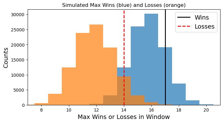
<p>In Figure 3, we show the results of 100,000 simulated runs of 
112 games.  In this case we took a fixed win probability of 
\(p=0.6\), simulated a stretch of 112 games, then found the 
largest number of wins (losses) in a 20 game window. We then 
repeated this 100,000 times.  The blue histogram in Figure 3 
represents the 100,000 max wins and the orange histogram gives 
the 100,000 max losses. I have also indicated the observed values 
(wins = 17, losses = 14).</p>

<p align="center">
  <img alt="Simulation" src="/images/blog/bball/sim_hist_fig.png" width="500" />
  <br />
    Fig 3:  <em>Max wins (blue) and losses (orange) in a 20-game window 
                in 100,000 simulated 112 game stretches assuming a 
                constant win probability of 0.6</em>
</p>

<p>So are the observed max wins/losses values consistent with a 
win value of \(p=0.6\)?  Well, yeah, kinda. They certainly 
fall within the respective histograms (although the losses 
seem to be a bit further out on the tail than the wins).
But ideally we would be able to calculate a probability for 
each \(p\).  So let’s do that!</p>

<p>Let’s focus on what we set out to calculate.  That is, we want 
to find the probability that the highest number of wins 
(or losses) in a 20 game window throughout the season exceeds 
some number \(k\).  So we’ll now run our simulations for a range 
of \(p\) values and calculate this number by simply counting 
the number of max values that equal or exceed \(k\).  So for 
wins, we will simulate our 100,000 seasons and find the most 
wins in a 20-game window for each.  We will then count how many 
of these are greater than or equal to 17, and divide by the total 
number of simulations to get a probability.  We can do the same 
for losses.</p>

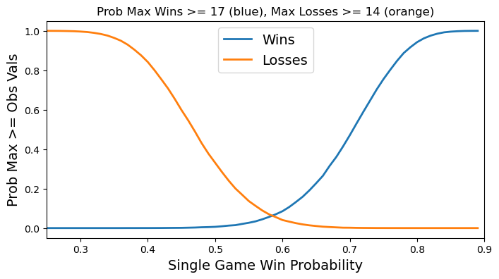
<p>Figure 4 below shows these results. The blue line gives the 
probability that the max number of wins in a 20 game window 
is greater than or equal to 17 for a range of win probabilities. 
Likewise the orange curve shows the probability that the max number 
of losses is greater than or equal to 14.</p>

<p align="center">
  <img alt="Sim" src="/images/blog/bball/sim_prob_fig.png" width="500" />
  <br />
    Fig 4:  <em>Probability that the max number of wins (blue) 
                and losses (orange) exceed the observed 
                values as a function of win probability.</em>
</p>

<p>These curves behave as we would expect.  If the win probability 
is very low, then the probability of getting a max of at least 
14 losses in a 20 game window is very good (i.e., 1). Likewise, 
if the win probability is very high, then the probability of 
getting a max of at least 17 wins in a 20 game window is very 
good (i.e., 1). However, it is odd that the intersection 
occurs at such a low probability (about 6%), but this could 
be evidence against our assumption that \(p\) is fixed 
for the whole season.</p>

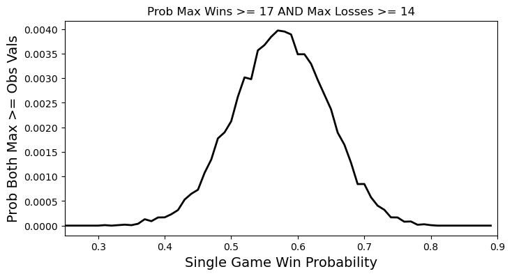
<p>Figure 4 showed the individual probability curves for losses 
and wins as a function of individual game win probability. But 
we want both of these to be true at the same time (since that’s what 
we saw).  To get the probability the max wins is greater than or 
equal to 17 <strong>and</strong> the max losses is greater than or equal to 14, 
we simply multiply the probabilities.  The result is shown 
below in Figure 5.</p>

<p align="center">
  <img alt="Sim" src="/images/blog/bball/sim_prob_prod_fig.png" width="500" />
  <br />
    Fig 5:  <em>Product of the two probability curves from Figure 4</em>
</p>

<p>This curve is a little noisy, but still looks about how we would expect 
by multiplying the two curves in Figure 4.  It has to go toward zero 
on the left because our blue curve goes to zero and it has to go toward 
zero on the right because our orange curve goes to zero.  It is maximum 
where the two curves from Figure 4 intersect.  The peak of this probability 
curve is around \(p=0.57\), which is very close to the cumulative winning 
fraction after 112 games from Figure 2. With this win probability, 
we would expect the team to win about 92 out of 162 games for the 
regular season. Not setting any records, but still pretty good.</p>

<h1 id="conclusions">Conclusions</h1>

<p>By simulating the results, we were able to numerically calculate 
the probability of the maximum number of wins (or losses) in a 
20 game window exceeding some particular value.  Based on this, 
we see that the Phillies season probably has not been super well 
described by a single unchanging win probability.  To properly 
evaluate that claim, however, we would need to do some kind of 
model comparison.</p>

<p>However, in the next part we will <em>not</em> be doing that!  Instead 
we will consider a fun (?) yet <strong>highly impractical</strong> way of 
calculating the desired probability without simulations.</p>

<!---
<p align="center">
  <img alt="Phanatic Phorsaken" src="/images/blog/bball/phanatic_si.jpg" width="400">
  <br>
    <em>Phrustration (Image Credit: si.com)</em>
</p>
-->
<div class="footnotes" role="doc-endnotes">
  <ol>
    <li id="fn:1" role="doc-endnote">
      <p>Unless otherwise noted, all the data will come from 
  <a href="https://www.baseball-reference.com">baseball-reference.com</a>. 
  For example, you can find the results for the Phillies season 
  <a href="https://www.baseball-reference.com/teams/PHI/2024-schedule-scores.shtml#team_schedule">here</a>. <a href="#fnref:1" class="reversefootnote" role="doc-backlink">&#8617;</a></p>
    </li>
  </ol>
</div>]]></content><author><name>Robert S. Wharton</name><email>rswharton95@gmail.com</email></author><category term="Baseball" /><category term="Markov Process" /><summary type="html"><![CDATA[There’s an old Mitch Hedberg joke that goes “rice is great if you’re really hungry and want to eat two thousand of something.” Baseball is kind of like that. You have 162 games in the regular season where nine batters will get 3-5 chances to hit each game per team. The chance of getting a hit ranges from about 10% (not very good player) to about 30% (very good player) for each attempt. Over the course of the long season, a player can string together a series of hits (hot streak) or a series of outs (cold streak). These streaks could be due to something the player is doing (with the intrinsic probability of a hit changing), but can often be explained by statistical variance (with a fixed probability).]]></summary></entry><entry><title type="html">Highest Point in Delaware</title><link href="https://rwharton.github.io/posts/2024/08/blog-post-5/" rel="alternate" type="text/html" title="Highest Point in Delaware" /><published>2024-08-24T00:00:00-07:00</published><updated>2024-08-24T00:00:00-07:00</updated><id>https://rwharton.github.io/posts/2024/08/blog-post-5</id><content type="html" xml:base="https://rwharton.github.io/posts/2024/08/blog-post-5/"><![CDATA[<p>There are 13 US states with <a href="https://en.wikipedia.org/wiki/List_of_U.S._states_and_territories_by_elevation">peak elevations</a> above 10,000 feet.
The state of Delaware is not one of them.
Not even close. <a href="https://en.wikipedia.org/wiki/Ebright_Azimuth">Ebright Azimuth</a>, 
the highest point in Delaware, tops out at 448 feet above sea level.
Around Christmas 2023, my brother and I reached the summit.
Next up, <a href="https://en.wikipedia.org/wiki/Britton_Hill">Britton Hill, Florida!</a></p>

<table>
  <thead>
    <tr>
      <th style="text-align: center"><img src="/images/azimuth.jpg" alt="alt text" title="Two Intrepid Mountaineers" /></th>
    </tr>
  </thead>
  <tbody>
    <tr>
      <td style="text-align: center">My brother and I after the arduous stroll up Ebright Road.</td>
    </tr>
  </tbody>
</table>]]></content><author><name>Robert S. Wharton</name><email>rswharton95@gmail.com</email></author><category term="Mountaineering" /><category term="Delaware" /><summary type="html"><![CDATA[There are 13 US states with peak elevations above 10,000 feet. The state of Delaware is not one of them. Not even close. Ebright Azimuth, the highest point in Delaware, tops out at 448 feet above sea level. Around Christmas 2023, my brother and I reached the summit. Next up, Britton Hill, Florida!]]></summary></entry><entry><title type="html">Tales from the Transit of Venus</title><link href="https://rwharton.github.io/posts/2012/06/old-blog-1/" rel="alternate" type="text/html" title="Tales from the Transit of Venus" /><published>2012-06-05T00:00:00-07:00</published><updated>2012-06-05T00:00:00-07:00</updated><id>https://rwharton.github.io/posts/2012/06/sad-old-sun</id><content type="html" xml:base="https://rwharton.github.io/posts/2012/06/old-blog-1/"><![CDATA[<p align="center">
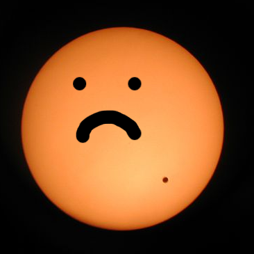
  <img src="/images/sad_transit.png" width="400" />
  <br />
    <em>Sad Old Sun</em>
</p>

<p>Today is the transit of Venus, which, aside from being a totally rad
astronomical event, is also the perfect excuse to tell my favorite story
of an unlucky Frenchman (I have many). This is by no means new and, if
you’ve ever taken an astronomy course, you’ve probably already heard it.
It is perhaps the closest thing Astronomy has to a ghost story, told
though the glow of a flashlight on moonless nights to scare the
children. This is the story of Guillaume Le Gentil, a dude that just
couldn’t catch a break.</p>

<!-- more -->

<p>Guillaume Joseph Hyacinthe Jean-Baptiste Le Gentil de la Galaisière was
a Frenchman with an incredibly long name. He was also an astronomer,
though he hadn’t started out that way. Monsieur Le Gentil (as his
friends called him and so, then, shall we) had originally intended to
enter the priesthood. However, he soon began sneaking away to hear
astronomy lectures and quickly switched from studies of Heaven to those
heavens more readily observed in a telescope. Le Gentil happened to get
into the astronomy game at a very exciting time. The next pair of Venus
transits was imminent and astronomers were giddy with anticipation.
Though the previous transit of 1639 had been predicted, it was met with
little fanfare and only a few measurements. But the transits of 1761 and
1769 would be different. People would be ready. And the stakes were
higher this time, too. Soon after the 1639 transit, Edmund Halley (he of
the-only-comet-people-can-name fame) calculated that with enough
simultaneous measurements, the distance from the Earth to the Sun (the
so-called astronomical unit, or AU) could be measured fairly accurately.
Since almost all other astronomical distances were known in terms of the
AU, knowing its precise value would essentially set the scale for the
cosmos. Brand new telescopes in hand, the astronomers of Europe set sail
for locations all over the world.</p>

<p>Le Gentil had been assigned to observe the transit from Pondicherry, a
French holding on the eastern side of India. On March 26th, 1760, he
began his long sea voyage around the Cape of Good Hope towards India.</p>

<p>The voyage from France to India was a bit too long for the ship Le
Gentil hitched a ride on and he only made it as far as Mauritius (a
small island off Madagascar). Dropped off with all his equipment, Le
Gentil was left waiting for any ship at all to take him to Pondicherry.</p>

<p>Perhaps it was the Curse of the
<a href="http://en.wikipedia.org/wiki/Dodo">Dodo</a> or perhaps it was just bad
luck, but while he was waiting, Le Gentil learned that
<a href="http://en.wikipedia.org/wiki/Seven_Years'_War">war</a> had broken out
between the French and the British, making a trip to British India very
difficult for a Frenchman.</p>

<p>Then the monsoon season started, meaning that even if he could find a
ship, it would have to take a much longer route to India than initially
planned and that it would be very difficult to make the journey before
the transit occurred.</p>

<p>Then, he caught dysentery for the first time.</p>

<p>Finally, after months of waiting, Le Gentil (barely recovered from his
illness) left Mauritius for India in February of 1761. Though time
appeared to be running out, the captain of the ship he was on promised
he would be there to observe the transit in June. About halfway to
India, the winds switched directions and the ship was forced to turn
back to Mauritius.</p>

<p>Le Gentil dutifully observed the transit of Venus in 1761 from a rocky
ship in the middle of the Indian Ocean. The data were useless and he
never attempted any analysis.</p>

<p>Although he missed the first transit, these things come in pairs
separated by eight years. There was still another chance. And with all
this time to prepare, there was no way he was going to miss the second
one.</p>

<p>In fact, there was a bit <em>too much</em> time. But as a world-traveling 18th
century man of science, Le Gentil had plenty of other interests to fill
his days. He was particularly interested in surveying the region around
Madagascar.</p>

<p>So he made a really nice map of Madagascar. And then he ate some bad
kind of some kind of animal and came down with a terrible sickness. He
describes this illness and its “cure” in his journals:</p>

<blockquote>
  <p><em>This sickness was a sort of violent stroke, of which several very
copious blood-lettings made immediately on my arm and my foot, and
emetic administered twelve hours afterwards, rid me of it quite
quickly. But there remained for seven or eight days in my optic nerve
a singular impression from this sickness; it was to see two objects in
the place of one, beside each other; this illusion disappeared little
by little as I regained my strength…</em></p>
</blockquote>

<p>After recovering from both his sickness and the treatment, Le Gentil
decided to begin his preparations for the 1769 transit of Venus. He
calculated that either Manila or the Mariana Islands would be the ideal
spot to observe. The Sun would be relatively high in the sky at both
places when Venus passed by, meaning that the view would be through less
atmosphere with a reduced chance of clouds passing through the line of
sight. Le Gentil packed up his stuff and headed off to Manila, where he
could catch another ship to get to the Mariana Islands. Arriving in
Manila in 1766, the astronomer found himself exhausted from months of
sickness and sea-voyage. So, when he was offered passage on a ship
heading to the Mariana Islands, he quickly declined. That he chose not
to depart Manila at that time was perhaps his one stroke of good luck in
the entire journey. The ship sunk. Writing in his journal, Le Gentil
appears to have developed that particular sense of humor that generally
accompanies constant disappointment:</p>

<blockquote>
  <p><em>It is true that only three or four people were drowned, those who
were the most eager to save themselves, which is what almost always
happens in shipwrecks. I cannot answer that I would not have
increased the number of persons eager to save themselves.</em></p>
</blockquote>

<p>In any case, Le Gentil was in Manila with plenty of time to prepare for
the next transit. Unfortunately, the astronomer may have over-prepared.
Having arrived three years before the event, he now had three years to
worry and second-guess his decision. It didn’t help that the Spanish
governor of Manila was kind of a crazy person. Not wanting to miss the
observation of a lifetime owing to the whims of mildly insane strong
man, Le Gentil packed up his stuff and headed to Pondicherry. Finally in
Pondicherry, Le Gentil worked tirelessly to construct his observatory
and make plenty of astronomical observations in preparation for the
event. He had state of the art equipment and had fully calibrated and
double checked everything. It was now nine years since his journey began
and only a few days until the transit was scheduled to occur at sunrise
on June 4th. The entire month of May was beautiful weather and pristine
observing conditions, as were the first few days of June. Le Gentil
likely went to bed on the 3rd of June fully confident that the next
morning would be no different. He woke up early in the morning to begin
preparations for his sunrise observations only to find clouds on the
horizon. The clouds remained, obscuring the sun, all through the
duration of the transit. A few hours after the end of the transit, the
sun broke through the clouds and remained visible for the rest of the
day. Le Gentil had missed his second transit in Pondicherry. He sums it
up in his journal:</p>

<blockquote>
  <p><em>That is the fate which often awaits astronomers. I had gone more
than ten thousand leagues; it seemed that I had crossed such a great
expanse of seas, exiling myself from my native land, only to be the
spectator of a fatal cloud which came to place itself before the sun
at the precise moment of my observation, to carry off from me the
fruits of my pains and of my fatigues</em></p>
</blockquote>

<p>In Manila, the Sun rose in perfectly clear skies. Distraught, Le Gentil
remained in bed for some weeks afterward. He soon caught a fever and
missed the ship that was supposed to take him home. He recovered, but
then came down with dysentery again. Barely recovered from his various
illnesses, he managed to get a ride back to Mauritius. He caught a ship
leaving the island in November of 1770. The ship was struck by a
hurricane and almost completely destroyed. It managed to limp back to
Mauritius. The second attempt proved more successful and Le Gentil
finally “set foot on France at nine o’clock in the morning, after eleven
years, six months and thirteen days of absence.” Though he had finally
made it home, he was not out of the woods quite yet. In his absence, Le
Gentil’s heirs had tried to declare him dead to gain their inheritance,
his accountant had mishandled (and lost) a large chunk of his holdings,
and the Academy of Sciences, which had sent him on his 11 year mission,
had given his seat to someone else. It was not quite the welcome home he
had hoped for. Despite his seemingly never-ending misfortune, things did
turn around for Le Gentil. He married, had a daughter, and was
reinstated into the Academy of Sciences. Presumably, he lived out the
rest of his days in relative happiness. Le Gentil died in 1792. Keeping
true to his style, this man who missed two of the most important
astronomical events of his time fortunately managed to also miss the
most important (and violent) <a href="http://en.wikipedia.org/wiki/Reign_of_Terror">political
event</a> of his time.</p>

<hr />

<p><strong>References:</strong></p>

<p>I have mainly used a very nice series of historical papers of Le
Gentil’s misadventures with the transit of Venus written by Helen Sawyer
Hogg. The papers were originally published in the <em>Journal of the Royal
Astronomical Society of Canada</em> and can be accessed through NASA’s ADS 
(<a href="http://adsabs.harvard.edu/abs/1951JRASC..45...37S">Part 1</a>, 
<a href="http://adsabs.harvard.edu/abs/1951JRASC..45...89S">Part2</a>, 
<a href="http://adsabs.harvard.edu/abs/1951JRASC..45..127S">Part 3</a>, 
<a href="http://adsabs.harvard.edu/abs/1951JRASC..45..173S">Part 4</a>).</p>

<p><strong>More Transit of Venus:</strong></p>

<p>If you want to see the Transit of Venus without having to go on an
eleven year voyage (or even leaving your room), check out the NASA
<a href="http://sunearthday.nasa.gov/transitofvenus/">live-feed</a> from Mauna Kea.</p>

<hr />

<p><em>This was originally published on an</em> <a href="https://thevirtuosi.blogspot.com/2012/06/tales-from-transit-of-venus.html">old blog</a> <em>I ran with other physics grad students.</em></p>]]></content><author><name>Robert S. Wharton</name><email>rswharton95@gmail.com</email></author><category term="Old Blog" /><category term="Venus" /><summary type="html"><![CDATA[Sad Old Sun]]></summary></entry><entry><title type="html">Futurama Physics</title><link href="https://rwharton.github.io/posts/2011/08/futurama" rel="alternate" type="text/html" title="Futurama Physics" /><published>2011-08-22T00:00:00-07:00</published><updated>2011-08-22T00:00:00-07:00</updated><id>https://rwharton.github.io/posts/2011/08/futurama</id><content type="html" xml:base="https://rwharton.github.io/posts/2011/08/futurama"><![CDATA[<p align="center">
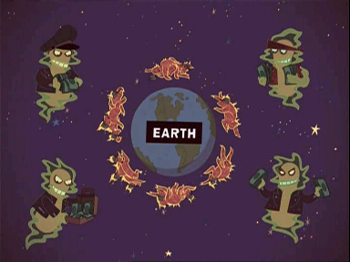
  <img alt="Global Warming" src="/images/blog/futurama/global_warming.png" width="400" />
  <br />
    <em>The cause of global warming.</em>
</p>

<p>Good news, everyone! I’m going to tell you about a fairly 
well-posed problem in <em>Futurama</em>.  In the episode “Crimes of 
the Hot,” all of the Earth’s robots vent their various “exhausts” 
into the sky at the same time, using the thrust to push the Earth 
into an orbit slightly further away from the sun. As a result of 
this new orbit, the year is made longer by “exactly one week.” 
Anything that quantitative is pretty much asking to be analyzed.</p>

<p>First, a little background. In this episode, it is learned that 
all the robots (especially Hedonism Bot) emit the greenhouse 
gases responsible for Global Warming. The previous solution (detailed
<a href="http://www.youtube.com/watch?v=2taViFH_6_Y">here</a>) is no longer viable,
so it is decided that all robots must be destroyed (especially Hedonism
Bot). The disembodied head of Richard Nixon rounds up all the world’s
robots on the Galapagos<sup id="fnref:1" role="doc-noteref"><a href="#fn:1" class="footnote" rel="footnote">1</a></sup> to have a “party” so that they may be
destroyed by a giant space-based electromagnetic pulse cannon. In a
last-ditch effort to save the robots, Professor Farnsworth has all the
robots blast their exhausts into the sky, using the thrust to push the
Earth into an orbit further away from the sun, thus solving the problem
of global warming once and for all. As a result of changing the Earth’s
orbit, the year is “exactly one week longer.”</p>

<h1 id="first-pass-through">First Pass Through</h1>

<p>Ok, so what can we say about the new orbit if all we know 
is that its orbital period is exactly one week longer? Well, 
we know from our good buddy Kepler that the square of the 
period of a bound orbit is proportional to the cube of its 
semi-major axis<sup id="fnref:2" role="doc-noteref"><a href="#fn:2" class="footnote" rel="footnote">2</a></sup>, so</p>

\[\tau^2 \propto a^3.\]

<p>We already know the Earth’s period (1 year) and semi-major axis 
(1<a href="http://en.wikipedia.org/wiki/Astronomical_unit">AU</a>) before the
robo-boost, so we can get rid of the proportionality by writing things
in terms of the initial values. In other words,</p>

\[\left(\frac{\tau}{1~\mbox{yr}}\right)^2=\left(\frac{a}{1~\mbox{AU}}\right)^3.\]

<p>Alright, so we know that our new orbital period is 1 year + 1 week, or
since there are 52 weeks in a year, 53/52 years. So our new semi-major
axis is</p>

\[a = \left(\frac{1 + 1/52~\mbox{yr}}{1~\mbox{yr}}\right)^{2/3}\mbox{AU}
    \approx1.013~\mbox{AU},\]

<p>or a little over 1% larger than it is currently. Fair enough. 
So would this fix Global Warming for ever and ever? Let’s see.</p>

<p>The solar flux at some distance \(d\) is given by</p>

\[S = \frac{L_{\odot}}{4\pi d^2},\]

<p>where L is the luminosity of the sun. So the ratio of the flux at the
new semi-major axis<sup id="fnref:3" role="doc-noteref"><a href="#fn:3" class="footnote" rel="footnote">3</a></sup> to that before the orbit was changed is</p>

\[\frac{S}{S_0}=\left(\frac{a_0}{a}\right)^2
             =\left(\frac{a}{1~\mbox{yr}}\right)^{-2}.\]

<p>OK, so we have the flux, but how do we relate this to temperature? 
Well, we know that the power radiated by a blackbody of temperature 
T is given by</p>

\[P = \sigma A T^4,\]

<p>where \(\sigma\) is the Stefan-Boltzmann
<a href="http://en.wikipedia.org/wiki/Stefan%E2%80%93Boltzmann_law">constant</a>, 
A is the area of the emitting region and T is the temperature. For a
blackbody in equilibrium, the power coming in is going to be equal to
the power going out. The power coming in is just the solar flux times
the cross-section area of Earth, given by</p>

\[P_{in} = S\times\pi R^2_{\oplus}\]

<p>and the power going out is just that radiated by the Earth as a blackbody</p>

\[P_{out} =\sigma \times 4\pi R^2_{\oplus}\times T^4.\]

<p>Equating the power in to the power out gives</p>

\[T = \left( \frac{S}{4\sigma}\right)^{1/4}.\]

<p>Now we can find the ratio of the new average Earth temperature 
to the temperature before the orbital move. We have</p>

\[\frac{T}{T_0} =\left(\frac{S}{S_0}\right)^{1/4}
              =\left(\frac{a_0}{a}\right)^{1/2}
              \approx0.994\]

<p>If we take the initial average Earth temperature to be something like 
\(T = 300~{\rm K}\), then we find a new temperature of \(T = 298~{\rm K}\). 
A whole 2 degrees cooler!</p>

<p>That may not sound like a lot, but remember, that’s the mean 
global temperature. Apparently, it only takes a few degrees 
increase in global average temperatures to make things uncomfortable 
for people. The IPCC
<a href="http://en.wikipedia.org/wiki/Global_warming">indicates</a> that the
average global surface temperature on Earth in the next century is
likely to rise by about 1 to 2 degrees under optimistic scenarios or
about 3 to 6 degrees under pessimistic scenarios. So the robo-boost
option is at least in the right ballpark here. Neat!</p>

<h1 id="how-big-is-the-push">How Big Is The Push?</h1>

<p>So how big of a push did the robots need to give the Earth to
boost it out to this new orbit? Is this possible? Let’s find out!</p>

<p>First we need to find out how the Earth’s velocity has changed. 
We can do this by finding the change in energy. The total energy 
of a bound orbit is given by</p>

\[E = -\frac{k}{2a}\]

<p>where \(a\) is the semi-major axis of the orbit and 
\(k= GMm\). So the difference in Earth’s energy before and
after the robo-boost is</p>

\[E_f - E_0 =-\frac{k}{2a_f}-\left(-\frac{k}{2a_0}\right)
          =\frac{k}{2a_0}\left(1-\frac{a_0}{a_f}\right).\]

<p>But we also know that Earth’s energy in the orbit is 
given by</p>

\[E = -\frac{k}{r} + \frac{1}{2}mv^2,\]

<p>so the difference in energy before and after is</p>

\[E_f - E_0 =\frac{1}{2}m\left(v^2_f-v^2_0\right),\]

<p>where we have found the energies immediately before and immediately 
after the boost so Earth is pretty much at the same distance from 
the sun, so the potential energy terms cancel. Combining our 
expressions for the change in energy and solving for the final 
velocity, we find</p>

\[v_f = \left[\frac{GM_{\odot}}{a_0}\left(1-\frac{a_0}{a_f}\right)+v^2_0\right]^{1/2}.\]

<p>Taking the initial orbital velocity of the Earth to be 30 km/s, we find
that the final velocity of the Earth immediately after the robo-boost is</p>

\[v_f = 30.2~\mbox{km/s}\]

<p>So the robots just need to give a “little” 200 m/s boost to the Earth, 
right? Well, we are adding velocity vectors here, so it depends on 
which direction the robots are pushing. The magnitude of the final 
velocity is given by</p>

\[v_f = \sqrt{\left({\bf v_0}+{\bf \Delta v}\right)^2}
      =\sqrt{v^2_0+\Delta v^2-2v_0\Delta v\cos{\beta}},\]

<p>where \(\Delta v\) is the boost in velocity caused by the
robots and \(\beta\) is the angle between the initial orbital 
motion of the Earth and the velocity boost from the robots.</p>

<p>If they wanted to make it slightly easier on themselves, 
the robots would have boosted the Earth in the direction it 
was already moving. That would make the \(\cos \beta\) term 
equal to one and thus minimize the necessary boost. However, in the
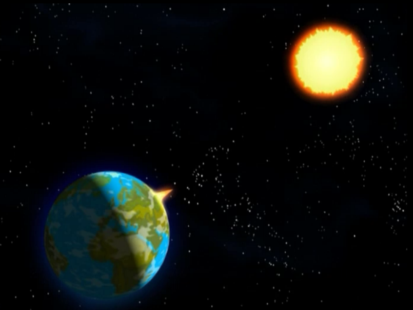
show the robots appear to point their exhaust right at the sun (see
figure below). This is essentially at a 90 degree angle to the Earth’s
orbital motion, so the \(\cos \beta\) term goes to zero in our 
expression above.</p>

<p>Plugging it all in we find that the magnitude of the robo-boost
is</p>

\[\Delta v \approx 3.5~\mbox{km/s}.\]

<p>We see that this is a fair bit larger than the 0.2 km/s 
needed for a boost parallel to Earth’s initial velocity.</p>

<p align="center">
  <img alt="Delta v" src="/images/blog/futurama/delta_v.png" width="400" />
  <br />
    <em>Robots blasting from the Galapagos (which now appear to be in China...)</em>
</p>

<p>Alright, so how much effort would it take to give that kind of boost to
the Earth? We can quantify this effort in terms of a force or in terms
of the energy difference. Let’s do both.</p>

<p>For the force, we have</p>

\[F = \frac{\Delta p}{\Delta t}=\frac{M_{\oplus}\Delta v}{\Delta t}.\]

<p>Here we are a little stuck unless we can figure out the duration of the
robo-boost. Watching the episode again, the robots are blasting up
exhaust for about a minute but then the show cuts to commercial. So we
don’t really know how long they were pushing. Let’s just say an hour,
but we’ll leave the time in if we want to fiddle with that.</p>

<p>Plugging in numbers, the total force is</p>

\[F = 6\times10^{24}~\mbox{N}\left(\frac{\Delta t}{1~\mbox{hr}}\right)^{-1}.\]

<p>If this force is spread evenly over the billion robots present<sup id="fnref:4" role="doc-noteref"><a href="#fn:4" class="footnote" rel="footnote">4</a></sup>, then 
each robot would be applying a force of</p>

\[F = 6\times10^{15}~\mbox{N},\]

<p>which is roughly equivalent to the force it would take to lift up 
Mount Everest<sup id="fnref:5" role="doc-noteref"><a href="#fn:5" class="footnote" rel="footnote">5</a></sup>.</p>

<p>That wasn’t terribly helpful. Let’s look at the work then 
instead. The total work done by the robots to move the Earth 
is</p>

\[W = \frac{1}{2}M_{\oplus}\left(v^2_f - v^2_0\right) 
     \approx 4\times10^{31}~\mbox{J}.\]

<p>Well, that’s a large number. Could a billion robots feasibly do that 
much work? If the robots are each 100 kg, then if the mass of all 
billion robots were directly converted to energy, we would get</p>

\[E = mc^2 = 10^9\times10^2~\mbox{kg}
           \times\left(3\times10^8~\mbox{m/s}\right)^2
         \approx 10^{28}~\mbox{J},\]

<p>or less than a thousandth the total energy needed. So it looks unlikely 
that the robots would be able to push the Earth, but that was to be 
expected.</p>

<h1 id="changes-to-the-orbit">Changes to The Orbit</h1>

<p>Let’s take a look at how the robo-boost affects the entirety of the
Earth’s new orbit. In our first pass through the problem, we ignored the
fact that the shape of the orbit changed and only focused on the new
semi-major axis. To see why we must also consider the changes to the
“shape” of the orbit, take a look at the figure below.</p>

<p align="center">
  <img alt="Orbits" src="/images/blog/futurama/orbits.png" width="400" />
  <br />
    <em></em>
</p>

<p>In the figure, the initial orbit is plotted (black dashed line) as well
as two new orbits that each have the appropriate semi-major axis so that
the period of revolution is one year and one week. The difference
between the two final orbits comes from the robots pushing in different
directions. In the blue orbit, the boost was made in a direction
radially outward from the Sun (that is, perpendicular to the orbital
velocity of the Earth). This is the case shown in the <em>Futurama</em> episode.
In the red orbit, the boost was made parallel to the orbital velocity of
the Earth. In each case, the boost was applied at the point labeled with
an “X.”</p>

<p>One thing that jumps out from this figure is that the Earth is
always further away from the sun on the red orbit than it was on the
initial (dashed black) orbit. But on the blue orbit, the Earth is
further away from the Sun than it was initially for only half the orbit.
On the other half, the blue orbit would actually make the Earth’s
temperature <em>higher</em> than it was on the old orbit!</p>

<p>The temperature calculation we made earlier should hold pretty well 
for the red orbit, since it is essentially a circle. It would be a 
little more tricky for the blue orbit, as one would need to get a 
time-averaged value of the flux over the course of the whole orbit. 
A hundred Quatloos to anyone that does the calculation.</p>

<h1 id="wrap-up">Wrap-Up</h1>

<p>So what have we found out here? Well, it seems that there are certain 
scenarios in which boosting the Earth out to a new orbit with period 
of 1 year + 1 week could cool the Earth by a few degrees. Granted, 
we have made some simplifications (the Earth is not a blackbody), 
but the general idea of the thing should still hold.</p>

<p>I had some fun playing around with this problem and I thought it
was neat that there was a good deal of information to get started with
from the episode. The <em>Futurama</em> people gave an exact period and at
least a visual representation of the direction the robots apply their
push. So 600 Quatloos for the writers!</p>

<p><em>This was originally published on an</em> 
<a href="https://thevirtuosi.blogspot.com/2011/08/futurama-physics.html">old blog</a> 
<em>I ran with other physics grad students.</em></p>
<div class="footnotes" role="doc-endnotes">
  <ol>
    <li id="fn:1" role="doc-endnote">
      <p>According to the Wikipedia page for the <a href="http://en.wikipedia.org/wiki/Crimes_of_the_Hot#Production">episode</a>, the location of the Galapagos for the party was chosen because the writers felt that it would be most convenient to push the Earth near the equator. <a href="#fnref:1" class="reversefootnote" role="doc-backlink">&#8617;</a></p>
    </li>
    <li id="fn:2" role="doc-endnote">
      <p>The semi-major axis of an ellipse is half of the longest line cutting through the center of the ellipse. Likewise, the semi-minor axis is half of the shortest line drawn through the center of the ellipse. Check <a href="http://mathworld.wolfram.com/Ellipse.html">this</a> out for some more fun stuff on ellipses. <a href="#fnref:2" class="reversefootnote" role="doc-backlink">&#8617;</a></p>
    </li>
    <li id="fn:3" role="doc-endnote">
      <p>This is technically incorrect, since the semi-major axis is measured from the center of the ellipse, but the sun is located on one of the foci. However, this requires information on the  eccentricity of the orbit, which we are currently glossing over right now. Our method is then approximate, but becomes exact in the case where both orbits are circles. The effect, however, is minor. At worst, it is semi-minor. <em>Zing!</em> <a href="#fnref:3" class="reversefootnote" role="doc-backlink">&#8617;</a></p>
    </li>
    <li id="fn:4" role="doc-endnote">
      <p>My source for this billion robots number comes from Professor Farnsworth himself. When it looks like the robots will all be destroyed the Professor says “A billion robot lives are about to be extinguished. Oh, the Jedis are going to feel this one!” <a href="#fnref:4" class="reversefootnote" role="doc-backlink">&#8617;</a></p>
    </li>
    <li id="fn:5" role="doc-endnote">
      <p>Well, sort of. The height of Everest is \(\sim 10^4~{\rm m}\), so this gives a volume of \(\sim 10^{12}~{\rm m}^3\). The density of most metals is around \(10 {\rm g/cm}^3\), which is \(10^4~{\rm kg/m}^3\). This gives a mass of \(\sim 10^{16}~{\rm kg}\). The weight is then \(\sim 10^{17}~{\rm N}\). Each robot exerts a force of \(\sim 10^{16}~{\rm N}\). So not quite, but hey it was the first thing I thought of and it almost worked out so I’m sticking with it! <a href="#fnref:5" class="reversefootnote" role="doc-backlink">&#8617;</a></p>
    </li>
  </ol>
</div>]]></content><author><name>Robert S. Wharton</name><email>rswharton95@gmail.com</email></author><category term="Old Blog" /><category term="Orbits" /><summary type="html"><![CDATA[The cause of global warming.]]></summary></entry><entry><title type="html">Beards and Pulsars</title><link href="https://rwharton.github.io/posts/2010/09/beards-pulsars/" rel="alternate" type="text/html" title="Beards and Pulsars" /><published>2010-09-27T19:56:00-07:00</published><updated>2010-09-27T19:56:00-07:00</updated><id>https://rwharton.github.io/posts/2010/09/beards-pulsars</id><content type="html" xml:base="https://rwharton.github.io/posts/2010/09/beards-pulsars/"><![CDATA[<p align="center">
  <img alt="Hulse" src="/images/hulse.jpg" width="200" />
  <br />
    <em>The bearded half of Hulse-Taylor</em>
</p>

<p>A few weeks ago I was on a bus going through Scranton and I read a
super-awesome fun fact regarding the Hulse-Taylor binary pulsar in
<em>Black Holes, White Dwarfs and Neutron Stars</em>. Sadly, I have since
forgotten it and left the book a few thousand miles away. So, let’s just
make up our own!</p>

<p>First, we need a little background. What the heck is a
pulsar? A pulsar is a rapidly rotating neutron star that beams
electromagnetic radiation towards us, which is how we can see them.
Typical rotation periods range from a millisecond to a few seconds. So
each time the pulsar rotates, we observe a blip when the radiation beams
towards us. Since these objects are additionally very stable rotators,
they are essentially very accurate clocks with which we may make
astronomical measurements.</p>

<p>So what’s the Hulse-Taylor binary pulsar? The
Hulse-Taylor binary is almost exactly what it sounds like: it’s a pulsar
binary where one of the pulsars is pointed towards earth. It was the
first binary of it’s kind discovered and offers a unique look into a
very high gravity environment. It also provided a very nice test for
General Relativity. General Relativity predicts that two orbiting
massive bodies should emit gravitational waves. This emission of
gravitational waves will then cause the orbit to decay and the two
bodies to move closer together. So does the Hulse-Taylor binary show
this? Take a look:</p>

<p align="center">
  <img alt="Oribital Decay" src="/images/orbital_decay.jpg" width="350" />
  <br />
    <em>Orbital Decay of B1913+16 (Image credit: wikipedia)</em>
</p>

<p>The data fit the prediction of general relativity perfectly! For this
discovery Hulse and Taylor shared the 1993 Nobel prize in Physics.</p>

<p>Now that’s all well and good, but I was promised some fun facts…? Ah, yes!
Well, we mentioned that the Hulse-Taylor binary orbit is decaying. It
turns out that the orbit is decaying at about 3.5 meters per year.
That’s pretty slow. Let’s put it into a more conventional speed, like
meters per second. So</p>

\[3.5 {\rm m/yr} = 
   3.5 {\rm m/yr} \times \frac{1 \rm year}{3.14\times 10^7 \rm s} = 
   1.1 \times 10^{-7} {\rm m/s}\]

<p>or, in less useful units,</p>

\[3.5 {\rm m/yr} = 110 {\rm nm/s}\]

<p>Great, so what to compare this to? Well, all
people who are in the know know that I am a manly man who gained the
ability to grow facial hair sometime after my sophomore year of college.
And since I have to pretend to be an upstanding member of society this
week, I happen to know the last time I shaved. Thus, a few simple
measurements and I can estimate how long hair takes to grow.</p>

<p>The last
time I shaved was three days ago and a quick eyeball measurement (sadly
I have no ruler) gives a facial hair length of about 2mm. Thus, a beard
grows at about 0.7 mm/day.</p>

\[0.7 {\rm mm/day} = 
   0.7 {\rm mm/day} \times\frac{10^{-3} \rm m}{\rm mm} 
       \times \frac{1 \rm day}{86400\rm s} = 
   8 {\rm nm/s}\]

<p>This is a universal speed constant, which we shall call the speed of beard. 
Or, bowing to our corporate sponsors, we shall call it 
“Gillette Mach 1.” So doing a quick division, we find that the rate at 
which theHulse-Taylor binary’s orbit is shrinking is roughly 14 times beard
speed, or in our commercial units, Gillette Mach 14 (a razor close shave!).</p>

<p>“Well,” I hear you cry (a bit disappointed…?), “that’s a <em>pretty</em> 
useless unit, but can’t we be <em>more</em> useless?” Yes, dear reader, we 
certainly can! We are currently at
<em><a href="http://www.youtube.com/watch?v=2xZp-GLMMJ0">Snuggie</a></em><a href="http://www.youtube.com/watch?v=0Ym65h1bmJ0"></a>
levels of uselessness right now, but I think we can just about bump it up to
<em><a href="http://www.youtube.com/watch?v=0ONJfp95yoE">Member of Congress</a></em>
useless if we try.</p>

<p>A furlong is a unit of length about 200 meters long.
A fortnight is a unit of time about 14 days long. Therefore, if we want
a speed we just…</p>

\[{\rm \frac{furlong}{ fortnight}} =   
 1 \frac{\rm furlong}{\rm fortnight} \times \frac{200 \rm m}{\rm furlong} \times
\frac{1 \rm fortnight}{14 \times 86400 \rm s} = 
 1.6 \times 10^{-4} \frac{\rm m}{\rm s}\]

<p>So the rate of decay of the Hulse-Taylor binary is:</p>

\[3.5 {\rm m/yr} = 
   1.1 \times 10^{-7} {\rm m/s} \times 
        \frac{1 \rm furlong/\rm fortnight}{ 1.6 \times 10^{-4} {\rm m/s}} = 
  7 \times 10^{-4} \frac{\rm furlong}{\rm fortnight}\]

<p>Hooray! So now we know the decay rate of
the Hulse-Taylor binary orbit in two horrible units: either 700
microfurlongs per fortnight or 14 times the speed of beard (AKA Gillette
Mach 14). Please write these in your copybooks now and forever commit
them to memory.</p>

<hr />

<p><em>This was originally published on an</em> <a href="https://thevirtuosi.blogspot.com/2010/09/beards-and-pulsars.html">old blog</a> <em>I ran with other physics grad students.</em></p>]]></content><author><name>Robert S. Wharton</name><email>rswharton95@gmail.com</email></author><category term="old blog" /><category term="pulsars" /><summary type="html"><![CDATA[The bearded half of Hulse-Taylor]]></summary></entry><entry><title type="html">How Long Will a Bootprint Last on the Moon?</title><link href="https://rwharton.github.io/posts/2010/01/moon/" rel="alternate" type="text/html" title="How Long Will a Bootprint Last on the Moon?" /><published>2010-01-01T00:00:00-08:00</published><updated>2010-01-01T00:00:00-08:00</updated><id>https://rwharton.github.io/posts/2010/01/boot-moon</id><content type="html" xml:base="https://rwharton.github.io/posts/2010/01/moon/"><![CDATA[<p align="center">
  <img src="/images/bootprint_buzz.jpg" width="350" />
  <br />
    <em>Buzz Aldrin's bootprint (source: Wikipedia)</em>
</p>

<p>A couple of months ago, I stumbled across a bunch of
<a href="http://lroc.sese.asu.edu/images/157">pictures</a>
of Apollo landing sites taken by one of the cameras onboard the Lunar
Reconnaissance Orbiter. The images have a resolution high enough that
you can resolve features on the surface down to about a meter. Looking
at the Apollo 17 <a href="https://science.nasa.gov/resource/lro-apollo-17-landing-site-lithograph/">landing
site</a>,
you can see the trails of both astronauts and a moon buggy. 
It’s pretty cool.</p>

<p>It also got me thinking about how long the landing sites would be
preserved. More specifically, I want to know how long Buzz Aldrin’s
right bootprint (shown, incidentally, to the left) will last on the
Moon. Since the Moon has no atmosphere, the wind and rain that would
weather away a similar bootprint here on Earth are not present and it
seems as though the print would last a really long time. But how long?
Let’s try to quantify it.</p>

<h2 id="pick-your-poison">Pick Your Poison</h2>

<p>Before we get going, we need to figure out what physical process would
be most important in erasing a bootprint from the Moon. Although the
Moon lacks the conventional “weathering” we experience on Earth (due to
wind, rain, etc), it does experience something called “<a href="http://en.wikipedia.org/wiki/Space_weathering">space
weathering</a>.” Space
weathering is the changing of the lunar surface due to cosmic rays,
micrometeorite collisions, regular meteorite collisions, and the solar
wind. Of these phenomena, the most apparent
and well-studied would be the meteorites which have covered the Moon in
craters. We adopt the meteorite impact as our primary means of wiping
out a bootprint and restate our question as follows:</p>

<p>“How long would it take for a meteorite to hit the Moon such that 
the resulting crater wipes out Aldrin’s right bootprint?”</p>

<h2 id="background">Background</h2>

<p>As it is currently
stated, we can answer our question if we knew the rate of formation and
size distribution of the craters on the Moon. We could count up all the
craters on the Moon (or a particular region of interest) and tabulate
their sizes. This would give us the size distribution. It would also
give us a headache and potentially drive us to lunacy
Luckily, someone has beat us to it.</p>

<p><a href="http://adsabs.harvard.edu/abs/1966MNRAS.134..245C">Cross (1966)</a> 
used images from the Ranger 7 and 8 missions to count craters and 
determine the size distribution of craters in three regions of the Moon. 
The data for the crater distribution in the Sea of Tranquility 
(where Apollo 11 landed) are given in the figure below. Cross found 
that in the Sea of Tranquility, the number of craters with diameters 
greater than X meters (per million square kilometers) is given by:</p>

\[N(d&gt;X) = 10^{10}\left(\frac{X}{1~\mbox{m}}\right)^{-2},\]

<p>which holds for craters with diameters between 1 meter and 10 
kilometers (see figure below).</p>

<p align="center">
  <img src="/images/crater_pl.png" width="350" />
  <br />
    <em>Figure 2 from Cross (1966)</em>
</p>

<p>We can also estimate the rate at which craters are formed from this
data. If we assume that the craters formed at a constant rate over the
age of the Moon (about 4 billion years), then we get about 2.5 craters
with diameters above 1 meter formed in a million square kilometer area
every year. This is a “crater flux” for the Moon. Written another way,
the crater flux in the Sea of Tranquility is</p>

\[F \approx 1~{\mbox{km}}^{-2} \frac{1}{4\times10^5~\mbox{yr}},\]

<p>so we get that roughly one crater with diameter greater than 1 meter 
is formed on a square kilometer of the Moon once every 400,000 years 
or so.</p>

<p>We now have enough information to do some simulations.</p>

<h2 id="simulation">Simulation</h2>

<p>I wrote up a code that simulates craters being formed on a 1 square 
kilometer patch of the Moon. A crater is randomly placed in the 
1 square kilometer region with a diameter pulled from the above 
distribution. The bootprint is placed at the center of the grid 
and craters are formed until we get a “hit.” At that point, the 
time is recorded and the run stops. As a sanity check, I thought 
it would be fun to just let the simulation run without caring if 
the boot was hit or not. By simulating the craters in
this way for 4 billion years, I should get something that looks like the
Moon at the present day. Here’s a 200 m square from my simulation:</p>

<p align="center">
  <img src="/images/mymoon_wticks.png" width="450" />
  <br />
    <em>Simulated distribution of craters</em>
</p>

<p>and here’s a picture of the same-sized region on the surface of the
Moon:</p>

<p align="center">
  <img src="/images/200sq_m_moon.jpg" width="350" />
  <br />
    <em>Actual Image of the Moon (Source: LRO)</em>
</p>

<p>Just eyeballing it, things look pretty good.</p>

<p>Now it’s time for the actual simulation. I ran the simulation 10,000 
times and tabulated the amount of time needed before the bootprint was hit. 
The figure below gives the
<a href="http://en.wikipedia.org/wiki/Cumulative_distribution_function">CDF</a> for
the hit times in the simulation. That is, for each time T, we find the
fraction of simulations in which the bootprint got hit in a time less
than or equal to T. The dashed lines in the plot indicate the amount of
time needed to pass for half of the simulations to have recorded a hit.
This time turns out to be about 24 billion years.</p>

<p align="center">
  <img src="/images/hit_cdf.png" width="500" />
  <br />
    <em>Cumulative Distribution Function of a Hit</em>
</p>

<h2 id="conclusions-and-caveats">Conclusions and Caveats</h2>

<p>Based on the simulations, the bootprint on the Moon would have about 
even odds of lasting at least 20 billion years <em>if</em> the primary means 
of destruction is through the formation of a crater from a meteorite. 
However, there are a few caveats that should be addressed. These deal 
with either the details of the simulation or the assumptions we have made. 
In the simulation, we just took at 1 km square patch of the moon and scaled 
back the “crater flux” accordingly. However, this does not fully account 
for all possible craters that can form. For example, our simulation would 
miss an event that hit 50 km away from the target, but had a diameter 
of 100 km. Obviously this would hit the target, but we are only seeding 
craters in the 1 square km region. This would mean that the actual lifetime 
of the bootprint would be less than our 24 billion year figure. Re-running 
with a 10km by 10km square region, we find a lifetime of 18 billion years. 
Thus, an increase in area by a factor of 100 only reduces the age by 25%. 
Considering areas much larger than this makes the simulation prohibitively 
slow, but the order unity effect does not seem too significant.</p>

<p>Additionally, we have made a number of assumptions. The big one is that we 
have assumed that the craters currently seen on the Moon were formed 
uniformly in time. In fact, a large fraction of the craters may have been 
formed when the Moon was still very young (see <a href="http://en.wikipedia.org/wiki/Late_Heavy_Bombardment">Late Heavy
Bombardment</a>). If
this were the case, we would have greatly overestimated the rate of
crater formation and thus underestimated the time needed to hit the
bootprint.</p>

<p>In spite of these caveats, let’s take our value of 20 billion
years to be accurate. What else can we say? Well, if we are right then
we are wrong because the Moon may not last that long (and it’s hard to
have bootprints on the Moon without a Moon). Current
<a href="http://en.wikipedia.org/wiki/Sun#Life_cycle">estimates</a> have that the
Sun will expand into a red giant and (potentially) destroy the Earth
(and the Moon) in about 5 billion years. So a record of the Apollo
astronauts’ boot sizes could potentially last as long as the Moon. Not bad.</p>

<hr />

<p><em>This was originally published on an</em> <a href="https://thevirtuosi.blogspot.com/2012/01/how-long-will-bootprint-last-on-moon.html">old blog</a> <em>I ran with other physics grad students. A half-hearted attempt has been made to replace dead links.</em></p>]]></content><author><name>Robert S. Wharton</name><email>rswharton95@gmail.com</email></author><category term="Old Blog" /><category term="Moon" /><summary type="html"><![CDATA[Buzz Aldrin's bootprint (source: Wikipedia)]]></summary></entry></feed>