Cold Streak Part 2: Counting
Published:
This is Part 2 in our ongoing exploration of the important question how bad can a good baseball team be? In Part 1, we solved the problem in a quick, easy, but approximate way by running a bunch of simulations. Here we will consider a slow, painful, but exact way of solving our problem by enumerating states.
The Problem
Although I will probably keep using the terminology of the baseball season example that motivated this problem, we are mostly interested in a mathematical problem and it is important to state it in such terms. From Part 1, we will state our problem this way:
Assume we have a binomial process that has two outcomes: a win or a loss. Let \(p\) be the probability of a win, so that \(1-p\) is the probability of a loss. For a list of \(N\) games, what is the probability that the highest number of wins (or losses) in any \(M\) game window is greater than or equal to \(k\).
Our goal is to calculate this probability for any given values of \(p\), \(N\), and \(M\).
Starting Small
To get our bearings, we will spend this post working through a small example where we can actually enumerate all the possible win loss combinations. Consider a season of \(N=5\) games where we will consider windows of size \(M=3\). A 5 game season could then look like this:
\[S = \texttt{WWLWL}\]where the Ws are wins and the Ls are losses. It will be more convenient later on to represent the wins with a 1 and losses with a 0 so that the same season would look like this:
\[S = 11010\]For a \(N=5\) game season, we can form three \(M=3\) game windows and count the wins:
\[\begin{align} W_1 = &110\hphantom{10} ~\rightarrow~\textrm{2 wins} \\ W_2 = &\hphantom{1}101\hphantom{0}~\rightarrow~\textrm{2 wins}\\ W_3 = &\hphantom{10}010 ~\rightarrow~\textrm{1 win} \\ \end{align}\]so the maximum wins in a 3-game window for this season is 2.
From this simple example, we can already learn some things about the more general case. Since each game has exactly two possible outcomes (0 or 1), there will \(2^N\) possible ways to generate a list of \(N\) 0s and 1s. That means that there are \(2^N\) possible seasons. We can also see that for an \(N\) game season, there will be \(N-M+1\) possible windows of length \(M\).
Representing Seasons
Coming back to the \(N=5\) case, we see that there are only \(2^5=32\) possible seasons (which is a lot easier to deal with than the \(2^{162} \sim 10^{49}\) possible combinations for a full 162-game season). This means that we can very easily just write down all of the possible \(N=5\) game seasons. An easy way to do this is to note that any string of 0s and 1s is just a binary number. Just like we can write the base-10 representation of a number as
\[42 = 4 \times 10^1 + 2 \times 10^0\]we can write its binary (base-2) representation as
\[101010 = 1 \times 2^5 + 0 \times 2^4 + 1 \times 2^3 + 0 \times 2^2 + 1 \times 2^1 + 0 \times 2^0\]So enumerating all \(N=5\) length lists of 0s and 1s is equivalent to writing down the binary representation of the numbers 0 (00000) to 31 (11111). This is a neat little trick that we will be taking advantage of later.
Enumerating Seasons
We can now enumerate all possible season results (i.e., all ways to write down a combination of 5 ones and zeros). The 32 possible seasons for \(N=5\) are thus:
\[\begin{array}{c} 00000 & 00001 & 00010 & 00011 \\[5pt] 00100 & 00101 & 00110 & 00111 \\[5pt] 01000 & 01001 & 01010 & 01011 \\[5pt] 01100 & 01101 & 01110 & 01111 \\[5pt] 10000 & 10001 & 10010 & 10011 \\[5pt] 10100 & 10101 & 10110 & 10111 \\[5pt] 11000 & 11001 & 11010 & 11011 \\[5pt] 11100 & 11101 & 11110 & 11111 \\[5pt] \end{array}\]Now we can just step through each of the three \(M=3\) length windows for each season and find the maximum number of 1s that occur. Since we only have 32 different seasons, we can just count this manually:
\[\begin{array}{c|c|c|c} 00000 & 00001 & 00010 & 00011 \\ 0 & 1 & 1 & 2 \\[5pt] \hline 00100 & 00101 & 00110 & 00111 \\ 1 & 2 & 2 & 3 \\[5pt] \hline 01000 & 01001 & 01010 & 01011 \\ 1 & 1 & 2 & 2 \\[5pt] \hline 01100 & 01101 & 01110 & 01111 \\ 2 & 2 & 3 & 3 \\[5pt] \hline 10000 & 10001 & 10010 & 10011 \\ 1 & 1 & 1 & 2 \\[5pt] \hline 10100 & 10101 & 10110 & 10111 \\ 2 & 2 & 2 & 3 \\[5pt] \hline 11000 & 11001 & 11010 & 11011 \\ 2 & 2 & 2 & 2 \\[5pt] \hline 11100 & 11101 & 11110 & 11111 \\ 3 & 3 & 3 & 3 \\ \end{array}\]Since our window size is 3, the only allowed max values are 0, 1, 2, and 3 (that is, you can’t win more than 3 times in 3 games, no matter how hard you try). Let’s count how many of the season have each of thse \(k\) values:
\[\begin{align} n(k=0) &= 1 \\ n(k=1) &= 8 \\ n(k=2) &= 15 \\ n(k=3) &= 8 \\ \end{align}\]Probability (Special Case)
Now let’s consider a special case where the probability of a win is 0.5. That means that we are equally likely to draw a 1 or a 0. It also means that all seasons are equally likely, with
\[p_{S} = p^N = (1/2)^N = 2^{-N}\]which for \(N=5\) means \(p_{S} = 1/32\) for all seasons. Since all season have equal probability in this special case, we can calculate the probability of getting specific \(k\) values by counting the number of seasons with those \(k\) values and dividing by the total number of all seasons, so
\[p(k) = \frac{n(k)}{2^N}\]and thus
\[\begin{align} p(k=0) &= 1/32 \\ p(k=1) &= 8/32 = 1/4\\ p(k=2) &= 15/32 \\ p(k=3) &= 8/32 = 1/4 \\ \end{align}\]So just by counting we could calculate the probability for each \(k\) value for \(N=5\), \(M=3\), and \(p=0.5\). But what about arbitrary win probabilities, \(p\)?
Probability (General Case)
The \(p=0.5\) case was a simple matter of counting, but what about general \(p\)? Well, it’s a tiny bit more complicated, but we can do that as well. The difference will be that the seasons are no longer equally likely. To see this consider \(p=0.99\) where you have a 99% chance of winning any game. Then surely winning all five and losing all 5 have very different chances of happening.
Let’s now calculate the probability of a particular season happening. Since the probability of getting a 1 (a win) is \(p_1 = p\), then the probability of getting a 0 (a loss) is \(p_0 = 1 - p\). Since the games are independent events, the probability of the season is just the product of the probabilities of the individual games.
So the probability of getting season \(01101\) is
\[\begin{align} P(01101) &= p_0 \cdot p_1 \cdot p_1 \cdot p_0 \cdot p_1 \\ &= p_1^3 \cdot p_0^2 \\ &= p^3 \,(1-p)^2 \end{align}\]From this example, we see that the probability of any given season is determined just by the total number of wins. If we call the number of wins \(s\), then the number of losses is \(N-s\) and the probability of that season is
\[P(s) = p^s \, (1-p)^{N-s}\]To calculate the probability of the \(k\) values, we can utilize the enumeration table above, but we can’t use the total counts for each \(k\) like we did before. This is because the probability of each season is no longer the same and so not all \(k=2\) (for example) are equally likely.
Instead, we will use the Law of Total Probability and write:
\[P(k) = \sum_{i=0}^{2^N} P(k | S_i) P(S_i)\]where the term \(P(k | S_i)\) is a conditional probability that means the probability of getting \(k\) assuming you are in season \(S_i\). So in words this statement means that the probability of getting max counts \(k\) is equal to the sum (over all possible seasons) of the probability of getting \(k\) in seasons \(S_i\) times the probability of getting season \(S_i\).
We know how to calculate \(P(S_i)\), but what about the other term, \(P(k | S_i)\)? With our lookup table, this is simple because it will 1 if \(k=k_i\) and zero otherwise. For the season \(01101\), we have a \(k=2\), so
\[P(k | 01101) = \begin{cases} 1, & k=2 \\ 0, & \text{otherwise} \end{cases}\]Now we have enough information to calculate the exact probabilites for each \(k\) value for any win probability \(p\). We just generate all the valid seasons, count the \(k\) value for each season, and compute the probability for the season based on \(p\). We then use the law of total probability to sum everything up. The results are shown below and compared to the results from simulations.
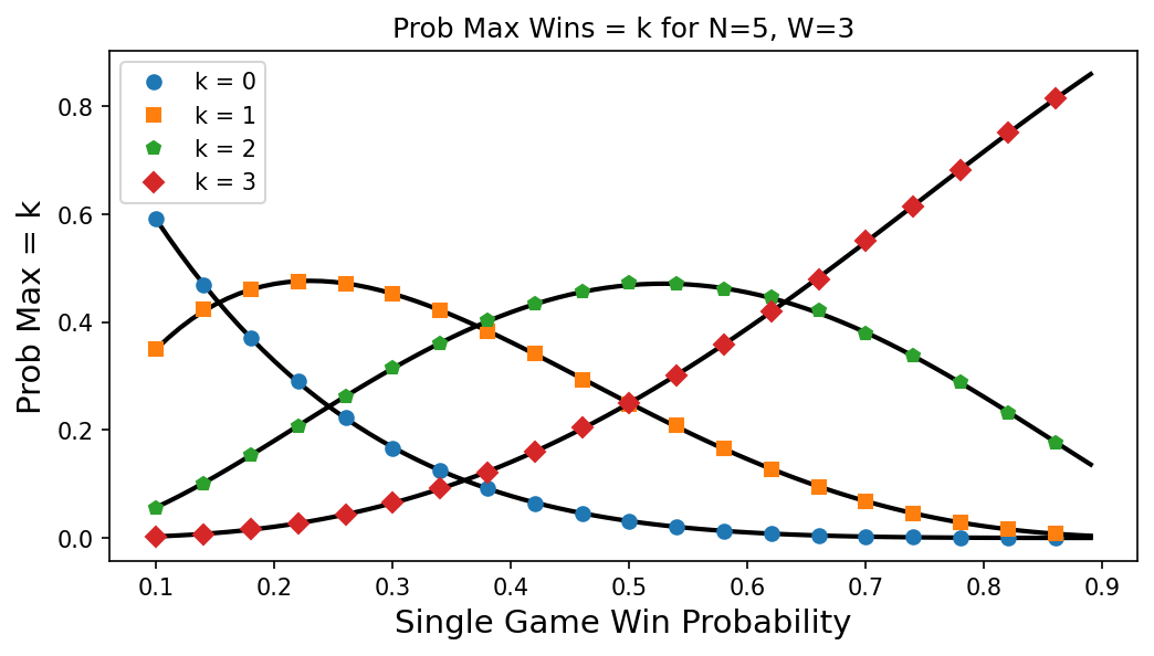
Fig 1: The curves show the exact probabilities calculated as described. The symbols show the probabilities estimated by the simulations we ran in Part 1.
Our calculated probabilities line up really well with the simulation results. The curves also behave as we would expect for varying values of individual game win probability \(p\). When \(p\) is very small, the lower \(k\) values dominate and then as \(p\) gets close to one, the higher values dominate. Also note that at \(p=0.5\), the probability of getting \(k=1\) is the same as \(k=3\), which we had found in our special case.
Conclusions
The purpose of this post was mostly to define some of our terms and hopefully gain some intuition for this problem. Enumerating all of the seasons in a small \(N\) case is useful for getting a sense of the problem but is a highly impractical means for getting an answer. For \(N=5\), we could pretty easily work with the 32 different seasons, but it was still tedious. As \(N\) gets bigger, this method not only becomes a pain, it also becomes impossible. You simply cannot list \(2^{162}\) different outcomes for a standard baseball regular season.
In Part 3, we’ll try a method that only requires us to keep track of the games in the running window of length \(M\). That’s something thats more practical. Well… maybe.