Cold Streak Part 3: Markov Chain
Published:
This is Part 3 of a series exploring a particular probability problem encountered while watching my baseball team lose (they got better). In baseball terms, the question was what is the maximum number of losses you expect a good team to have in any 20-game stretch during the season. In mathematical terms, the problem can be stated as
Assume we have a binomial process that has two outcomes: a win or a loss. Let \(p\) be the probability of a win, so that \(1-p\) is the probability of a loss. For a list of \(N\) games, what is the probability that the highest number of wins (or losses) in any \(M\) game window is greater than or equal to \(k\).
In Part 1, we were able to answer this question for particular \(N\), \(M\), \(k\), and \(p\) by simulating a large number of seasons and counting the max values. It wasn’t an exact solution, but was pretty easy. In Part 2, we took a very different approach. We considered the very small case of \(N=5\) and \(M=3\) and wrote down all possible seasons. From this we could calculate the exact probabilites for all \(k\) values for any single game win probability \(p\). This is exactly what we want… except that this method quickly becomes impossibly complex.
In this Part 3, we will use what we learned in Part 2, but avoid enumerating all \(2^N\) possible season results. Instead, we will only keep track of the \(2^M\) possible results within a window. For \(N=162\) and \(M=20\), this means “only” having to enumerate \(\sim10^6\) states instead of the full \(\sim10^{49}\). Progress!
Markov Process
First, we will need to learn a little something about Markov processes. A Markov process is a certain type of random process that generates a series of events. In a simple case, let’s say we have two states: A and B. At each step, we can either transfer between the states or stay in the current state. A key property of Markov chains is that the transition probabilities depend only on the current state, so all that matters is if we are currently in state A or B.
To generate a list of events with the Markov process, we simply look at what state we are currently in, then draw the next state based on the transition probabilities. For our simple example, lets say that when we are in state A, we can switch to state B with probability \(p_{\rm AB} = 0.2\) or stay in state A with \(p_{\rm AA} = 0.8\). When we are in state B, we can transfer to state A with probability \(p_{\rm BA} = 0.6\) or stay in state B with \(p_{\rm BB} = 0.4\).
If we start in state A, we can follow these rules to produce:
\[\texttt{A A B B A A B A A A B}.\]Transition Matrix
We can also write the probilities in the form of a transition matrix (or stochastic matrix). Each element of the transition matrix, \(p_{ij}\), will give the probability of going from state \(i\) to state \(j\). If we call states A and B states 0 and 1, we can write:
\[\begin{pmatrix} p_{00} & p_{01} \\ p_{10} & p_{11} \\ \end{pmatrix} = \begin{pmatrix} p_{AA} & p_{AB} \\ p_{BA} & p_{BB} \\ \end{pmatrix} = \begin{pmatrix} 0.8 & 0.2 \\ 0.6 & 0.4 \\ \end{pmatrix}\]Though it may take a little getting used to, the transition matrix description of a Markov process will make our lives much easier when we start calculating things. Let’s start with an easy example.
If we start in State A, what are the probabilites that we are in each state after one step? Since it’s just one step, we know that the answers are just \(p_{AA}\) for state A and \(p_{AB}\) for state B. But we can also calcualte this with the transition matrix:
\[\begin{align} \begin{pmatrix} p_A & p_B \\ \end{pmatrix} &= \begin{pmatrix} 1 & 0 \\ \end{pmatrix} \begin{pmatrix} p_{AA} & p_{AB} \\ p_{BA} & p_{BB} \\ \end{pmatrix}\\ &= \begin{pmatrix} 1 \cdot p_{AA} + 0 \cdot p_{BA} & 1\cdot p_{AB} + 0 \cdot p_{BB} \\ \end{pmatrix}\\ &= \begin{pmatrix} p_{AA} & p_{AB} \\ \end{pmatrix} \\ &= \begin{pmatrix} 0.8 & 0.2 \\ \end{pmatrix} \end{align}\]We can also do the same thing starting from state B:
\[\begin{align} \begin{pmatrix} p_A & p_B \\ \end{pmatrix} &= \begin{pmatrix} 0 & 1 \\ \end{pmatrix} \begin{pmatrix} p_{AA} & p_{AB} \\ p_{BA} & p_{BB} \\ \end{pmatrix}\\ &= \begin{pmatrix} 0 \cdot p_{AA} + 1 \cdot p_{BA} & 0\cdot p_{AB} + 1\cdot p_{BB} \\ \end{pmatrix}\\ &= \begin{pmatrix} p_{BA} & p_{BB} \\ \end{pmatrix}\\ &= \begin{pmatrix} 0.6 & 0.4 \\ \end{pmatrix} \end{align}\]where in each case we have specified the starting state via a row vector. I have gone through the operations to make clear how to multiply this with a matrix from the right. It’s a little different from what we typically see, but is just based on how the transition matrix is defined (you could make it a left transition matrix and operate on vectors by flipping rows and columns).
Many Steps
One of the nice things about the transition matrix approach is that it allows us to calculate probabilities at step \(n\) fairly easily. Based on what we saw above for a single step, multiple steps can be calculated by repeated multiplications of the transition matrix. This is equivalent to a single multiplication of the transition matrix to the \(n\)-th power:
\[P^n = \begin{pmatrix} p_{AA} & p_{AB} \\ p_{BA} & p_{BB} \\ \end{pmatrix}^n \\\]We can now easily calculate this matrix for any \(n\) for the problem above. We have
\[\begin{align} P^1 &= \begin{pmatrix} 0.8 & 0.2 \\ 0.6 & 0.4 \\ \end{pmatrix} \\ P^2 &= \begin{pmatrix} 0.76 & 0.24 \\ 0.72 & 0.28 \\ \end{pmatrix} \\ P^3 &= \begin{pmatrix} 0.752 & 0.248 \\ 0.744 & 0.256 \\ \end{pmatrix} \\ &\vdots \\ P^{10} &= \begin{pmatrix} 0.75 & 0.25 \\ 0.75 & 0.25 \\ \end{pmatrix} \\ \end{align}\]where we see something interesting happening. As we get more and more steps, the rows of the matrix converge to the same values. This means the the probability of being in a given state is independent of the starting value. We can see this beter in a plot:
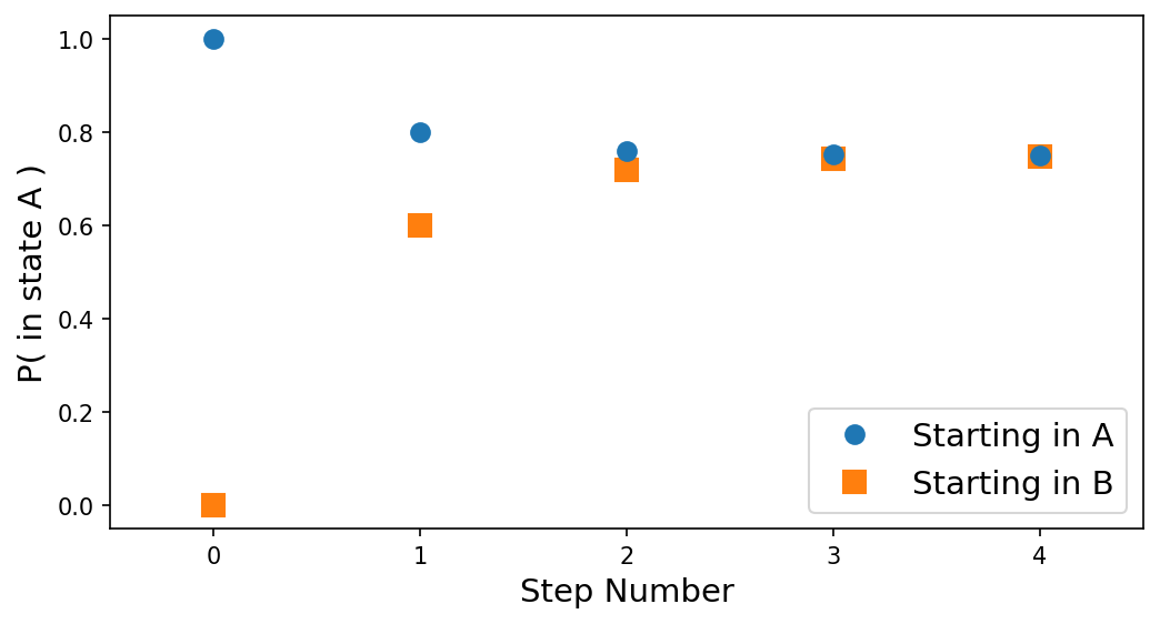
Fig 1: Probability of being in state A after n steps assuming we start in state A (blue circle) or state B (orange square)
This makes sense because the early steps will be affected by where we start, but eventually we get far enough away that we reach a steady state.
Absorbing State
Now what would happen if we added a third state C, that would only transition to itself (\(p_{CC} = 1\))? Since it does not allow transitions to other states, the chain would get stuck in C. For this reason, these states are called “absorbing states”.
Let’s modify our example above to include an absorbing state. Consider the transition matrix:
\[P = \begin{pmatrix} 0.7 & 0.2 & 0.1 \\ 0.5 & 0.3 & 0.2 \\ 0 & 0 & 1 \\ \end{pmatrix}\]which means A goes to \((A, B, C)\) with probability \((0.7, 0.2, 0.1)\), B goes to the same with probability \((0.5, 0.3, 0.2)\) and C only goes to C.
Since all states can go to C, but once there cannot leave, then eventually everything will go to state C. We can see this by calculating the result after, say, 10 steps:
\[P^{10} \approx \begin{pmatrix} 0.20 & 0.07 & 0.73 \\ 0.17 & 0.06 & 0.77 \\ 0 & 0 & 1 \\ \end{pmatrix}\]and after 20:
\[P^{20} \approx \begin{pmatrix} 0.05 & 0.02 & 0.93 \\ 0.04 & 0.01 & 0.94 \\ 0 & 0 & 1 \\ \end{pmatrix}\]where each row indicates the probability of being in states \((A, B, C)\) for starting state \(A\) (top row), \(B\) (middle row), and \(C\) (bottom row).
Absorbing states are useful for indicating a stopping condition, since once they reach that state, nothing changes. This is exactly what we will use an absorbing state for.
Back to Baseball
Now that we have a bit of background on Markov processes, let’s see if we can apply it to the problem at hand. Once again, our problem is
Assume we have a binomial process that has two outcomes: a win or a loss. Let \(p\) be the probability of a win, so that \(1-p\) is the probability of a loss. For a list of \(N\) games, what is the probability that the highest number of wins (or losses) in any \(M\) game window is greater than or equal to \(k\).
So we want to keep track of the number of wins (or losses) in a running window of \(M\) games. But that depends on the current game and the \(M-1\) previous games. The one rule we learned about a Markov process is that it is memoryless and can only depend on the current state. That is true, but we can be tricky about what we call a state.
Picking A State
One potential option is to enumerate every single possible combination of \(1\)s and \(0\)s in an \(M\) game window. From Part 2, we know that there are \(2^M\) ways to make a length \(M\) string of \(0\)s and \(1\)s. That could potentially get pretty unwieldy for large \(M\), but it sure beats enumerating every result in the season like we did in Part 2. But does it satisfy the Markov condition?
A Markov process has to be memoryless, which means that the transition properties can only depend on the current state. Let’s say that we have \(M=5\), then one of our states will be
\[s_i = 01101.\]The next possible state is just the string of 5 bits you get by shifting the window over one game. So for this state, the possible next states are:
\[s_{i+1} = \begin{cases} 11010, & \text{if next value is 0} \\ 11011, & \text{if next value is 1} \end{cases}\]because by moving our window one game over, we have lost the trailing \(0\) and picked up either a \(0\) or a \(1\).
We can also very easily calculate the transition probabilities are because it is simply the probability of getting a one, \(p\), or getting a zero \(1-p\). Thus the transition probabilities only depend on the current state, which satisfies the Markov condition.
Transitions
Since we are enumerating all \(2^M\) possible combinations for the contents of our length \(M\) window, we are going to have to be very careful about bookkeeping. If \(M=20\), we will have \(2^{20} \approx 10^6\) possible states. That’s too many to go through and identify by hand. Fortunately, we can use a clever trick we found in Part 2.
A simple way to enumerate all the \(2^M\) strings of zeros and ones is to simply count to \(2^M\) in binary (pre-pending zeros as necessary). So for \(M=5\) we would have
\[\begin{align} 0 &= 00000 \\ 1 &= 00001 \\ 2 &= 00010 \\ \vdots & \\ 29 &= 11101 \\ 30 &= 11110 \\ 31 &= 11111 \end{align}\]This means that we could keep track of each state by recording the base-10 number the corresponds to the binary string. This makes things much easier. Now, instead of storing, for example, a 15 game string of wins and losses as
\[s_i = 111101010110111\]we can instead just store the number
\[s_i = 31415\]Not bad!
But is there any way to figure what states this can transition to? Consider the state:
\[s_i = 11101.\]It can transition to the following states:
\[s_{i+1} = \begin{cases} 11010, & \text{if next value is 0} \\ 11011, & \text{if next value is 1} \end{cases}\]We described this in terms of shifting the \(M\) game window, but if we take the binary represenation seriously, then shifting one spot to the left is the same as multiplication by 2. As our window moves one spot right, all the numbers move one spot to the left, meaning one higher power of two. Now, there is a little bit of a catch because we are dropping the previously leftmost value. But that’s not a problem because we can just calculate the number modulo \(2^M\). The modulo is simply the remainder after dividing by \(2^M\). Since all of our states are by construction less than \(2^M\), this will give us what we want.
Let’s give it a try. The state \(s_i = 11101\) is the binary representation of the (base-10) number 29. So:
\[(29 \times 2) \mathbin{\rm mod} 2^5 = 58 \mathbin{\rm mod} 32 = 26\]and 26 in binary is \(11010\), which is indeed one of the answers that we were looking for. Since we are mutliplying by 2 and taking the modulo with respect to another even number, the result here will always be even. But the other valid state is exactly the same except the last bit is a 1. That means you just have to add one.
This means that for a given state \(s_i\) in base-10 representation, we can calculate the valid transitions as:
\[s_{i+1} = \begin{cases} 2 s_i \mathbin{\rm mod} 2^M, & \text{newest val a 0} \\ 2 s_i \mathbin{\rm mod} 2^M + 1, & \text{newest val a 1} \end{cases}\]and the probability of making these transitions is just \(p\) if the newest value is a one and \(1-p\) if the newest value is a zero.
Stopping Condition
Now that we have a neat way to represent our states, we should really go back to the problem. What is it we are trying to do again? We want to find the probability of getting at least \(k\) wins (or losses) in any \(M\) length stretch of games in an \(N\) length season. Therefore once we hit a state with \(k\) or more wins, we can stop, since our season has already met the goal. This sounds like the perfect case for an absorbing state!
For any value of \(k\), we will have some states that have less than \(k\) wins and others that will have at least \(k\) wins. The latter states are really just one state then. That is, they are the state where we have met our goal. If we call the states with less than \(k\) wins “valid” states then the total number of states we need to consider are \(n_{\rm valid} + 1\). This number will be less than \(2^M\), but will still be roughly the same order of magnitude.
Building the Transition Matrix
To build our transition matrix, we need to calculate \(p_{ij}\) between all possible states. But as we have seen above, any given state can transition to 2 other states with probability \(p\) if it ends in \(1\) or \((1-p)\) if it ends in 0. That means that most of our transition matrix will have rows that are mostly zero, but with two nonzero entries. The final absorbing state, however, will be all zeros except for a single entry of \(1\).
Previously we showed that any given state could be represented as a binary string which could then be turned into a base-10 number. We could then just index each state by this base-10 number, which would be pretty easy. However, some of these states will have have at least \(k\) wins and so would be absorbing states. We need to just have one absorbing state, so we will have to map all of these to the same index. This means we lose the easy indexing of states and are required to do one extra step where we map the base-10 number to the index value.
OK, so let’s try building the case where \(N=5\), \(M=3\), and we want \(k \geq 2\). For simplicity, let’s set \(p=0.5\). The valid states will have no more than 1 win. For \(M=3\), there are only 4 valid states:
\[\begin{align} 0 &: 000 \\ 1 &: 001 \\ 2 &: 010 \\ 4 &: 100 \\ \end{align}\]since any other state would have at least 2 ones. We then add one absorbing state to get a total of 5 possible states for this process.
\[P = \begin{pmatrix} 0.5 & 0.5 & 0 & 0 & 0 \\ 0 & 0 & 0.5 & 0 & 0.5 \\ 0 & 0 & 0 & 0.5 & 0.5 \\ 0.5 & 0.5 & 0 & 0 & 0 \\ 0 & 0 & 0 & 0 & 1 \\ \end{pmatrix}\]The first row is for \(000\), which can only transition to \(000\) (if the next val is a 0) or \(001\) if the next value is 1. The second row is for \(001\) which can only go \(010\) or \(011\), which has two wins and thus goes to the absorbing state. The third row is for \(010\), which can go to \(100\) or \(101\), which has two wins and thus also goes to the absorbing state. The fourth row is for \(100\) which can go to \(000\) or \(001\). The fifth row is the absorbing state, which can only go to itself with probability 1.
Calculating the Probability
Now that we have our transition matrix, we know how to calculate the probability that our system is in a given state after \(n\) steps. That would just be \(P^n\). But the way we have defined our states and the way we constructed our transition matrix means that we do not account for the starting point. We start with a state of \(M\) games. That means two things. First, we only need to propagate our system through \(N-M\) steps. Second, it means that we need to calculate the probability of starting in each given state.
Following with our simple example, if we want to calculate the probability that we start with state \(000\) and it ends up with \(k\geq2\), then we would do
\[P(s_0 = 000, k\geq2) = P(s_0 = 000) \cdot P(k\geq2 | s_0 = 000)\]In Part 2, we showed that the probability of getting \(n_0\) zeros and \(n_1\) ones in a string of length \(M\) is
\[P(s_i) = p^{n_1} (1-p)^{n_0}.\]For the absorbing state, its a little bit different because it encompasses all states with at least \(k\) ones. But for that we can use the binomial distribution:
\[P(s_4) = P(\geq k) = \sum_{s=k}^{M} {M\choose s} p^s (1-p)^{M-s}.\]The probability of getting \(k\geq 2\) at least once for each starting state can be read off from the final \(N-M\) step transition matrix, \(P^{N-M}\), in the last column in the row corresponding to the initial state.
For the transition matrix above with \(N=5\), \(M=2\), and \(p=0.5\), we have
\[P^{5-3} = P^2 = \begin{pmatrix} 0.25 & 0.25 & 0.25 & 0 & 0.25 \\ 0 & 0 & 0 & 0.25 & 0.75 \\ 0.25 & 0.25 & 0 & 0 & 0.50 \\ 0.25 & 0.25 & 0.25 & 0 & 0.25 \\ 0 & 0 & 0 & 0 & 1 \\ \end{pmatrix}\]So the final answer will be the sum over all states of the probability of starting in the state times the probability of that state ending in the absorbing state. That is:
\[P(k\geq 2) = \sum_{i=0}^{4} P(s_i) P^2_{i4}\]We would then get:
\[\begin{align} P(k\geq 2) = & \left[ (0.5^3) (0.25) \right]_{000} \\ & + \left[ (0.5^2 \cdot 0.5) (0.75) \right]_{001} \\ & + \left[ (0.5^2 \cdot 0.5) (0.50) \right]_{010} \\ & + \left[ (0.5^2 \cdot 0.5) (0.25) \right]_{100} \\ & + \left[ (3 \cdot 0.5^2 \cdot 0.5 + 0.5^3) (1) \right]_{\rm absorb} \\ = & \frac{23}{32} \end{align}\]In Part 2 we found that the probability of getting exactly 2 wins was \(15/32\) and the probability of getting exactly 3 wins was \(1/4\). Summing those gives a probability for \(k\geq 2\) of \(23/32\), which is exactly what we have here. That’s good!
What Have We Done?
This part ended up being a bit longer than I expected, so maybe it is useful to stop here and take stock of where we are. We developed a way to calculate the answer to our question using methods for Markov processes. For arbitrary values of \(N\), \(M\), \(k\), and \(p\) we can in principle enumerate the states, construct a transition matrix, and then finally calculate the total probability of getting at least one \(M\) game window with \(k\) or more wins.
This is an important achievement over our initial simulations because (up to numerical error), we know that the result we get will be exactly correct. However, this is still just a calculation, we have not found an equation to just plug in our parameters and get an answer. Instead we just have a method of getting the answer without any of the insight of an equation.
There is one big remaining problem, though. Our test case was the very small example we were able to previously work out by hand. Our calculation here requires a transition matrix that will be roughly \(2^M \times 2^M\) in size and we need to then calculate the \(N-M\)-th power of that matrix. At some point we are going to run into some performance issues. But we’ll deal with that next time!