Quantifying A Cold Streak
Published:
There’s an old Mitch Hedberg joke that goes “rice is great if you’re really hungry and want to eat two thousand of something.” Baseball is kind of like that. You have 162 games in the regular season where nine batters will get 3-5 chances to hit each game per team. The chance of getting a hit ranges from about 10% (not very good player) to about 30% (very good player) for each attempt. Over the course of the long season, a player can string together a series of hits (hot streak) or a series of outs (cold streak). These streaks could be due to something the player is doing (with the intrinsic probability of a hit changing), but can often be explained by statistical variance (with a fixed probability).
The same thing can happen when we consider the team as a whole. A team that wins 100 out its 162 games is very good (usually enough to win the division). However, this is only a winning percentage of about 62%. Better than flipping a coin, but not by a whole lot. So again, just by statistical chance, you could get hot streaks (win a bunch) or cold streaks (lose a bunch). But it is also possible that the team is just getting better or worse. Is there a way to tell the difference? Can we quantify when to panic?
Motivation
This exercise is mostly motivated by watching the ups and then sustained downs of my team, the Philadelphia Phillies. After getting out to a really hot start, the team started losing a lot more often in July and into August. Despite continuing to have one of (if not the) best record in baseball, fans started to panic. Sensing an opportunity to smugly explain this away as statistical variance, I took a look at the numbers1.
Grabbing the results for the 112 games at that point from baseball-reference.com, we can get a sense for how things changed over the course of the season (to that point). First we can plot the cumulative win fraction for the season. That is, for each game, we add up all the wins to that point and divide by the total number of games to that point. This will vary a lot early on because each game counts for more of the average, but will eventually steady out as each game is relatively less and less important. The results are shown in the next plot:
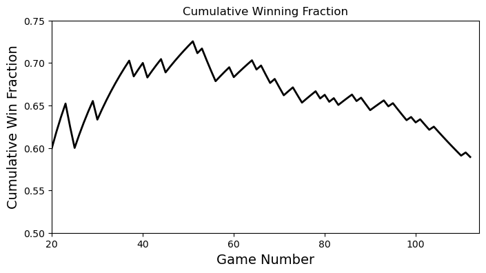
Fig 1: Cumulative win rate for the season
which tracks with experience. To get a sense for how good that peak is, note that only 15 teams have finished a season with a winning percentage above 70% (see here).
But if we are looking for ups and downs, maybe it is better to consider stretches of games. For example, we can check the win fraction for a rolling 20-game window. That is, we look at the last 20 games and calculate the fraction of games that were wins. We then go to the next game and do the same. This means that at each step we are adding the most recent game and removing the last game in the window. The results are shown in the following plot:

Fig 2: Winning Rate in a rolling 20 game window
This plot certainly tracks with how the season has felt. The team got off to a very hot start, then eventually started cooling off and losing more and more games.
Now we can finally get to the point: the highest win rate for a 20 game stretch this season is 0.85 and the lowest is 0.30. Are these consistent with a good team that will win 95-100 games?
The Problem
Let’s try to state the problem mathematically. Assume we have a binomial process that has two outcomes: a win or a loss. Let \(p\) be the probability of a win, so that \(1-p\) is the probability of a loss. For a list of \(N\) games, what is the probability that the highest number of wins (or losses) in any \(M\) game window is greater than or equal to \(k\). For Figure 2, we have \(N=112\) and \(M=20\). The max number of observed wins in a window is 17 and the max number of observed losses in a window is 14. We want to determine if these are statistically significant deviations for some given winning probability of \(p\).
Note that rolling \(M\) game window makes things a little tricky. If we had just said What is the probability that we get k or more wins in a list of M games?, then the solution would be given by the binomial distribution, which we could easily calculate. If we were considering independent groups of \(M\) games, we could calculate the probility for one and then use the binomial distribution again to calculate over the full season.
What makes our problem tricky is that, while the games themselves are independent, the counts in the rolling \(M\) game window are not independent. We can see this by considering a 20 game window that has 15 wins. When we shift over to the next game, we lose the least recent game (which could have been a win or a loss) and gain the most recent game (which again could be a win or a loss). That means that the number of wins in this window is constrained. It could only be 14 (if you drop a win and gain a loss), 15 (if the result you drop is the same you gain), or 16 (if you drop a loss and gain a win). To state it a bit more clearly, the number of wins in the current 20 game window depends on the current game and the previous 19.
An Easy Solution
If we just want to get an answer, we could just run a bunch of simulations and tally the results. This is what I did first, so let’s give it a try. A binomial process is very easy to simulate, so long as we have a way of generating a random number that is uniformly distributed on the interval \([0, 1)\). If we draw a number \(d\) in this interval, we will consider the event a win if \(d\leq p\), otherwise it’s a loss. Doing this \(N\) times gets us a season. Once we generate a season, we can loop through and find the max wins and losses in a rolling 20 game window.
In Figure 3, we show the results of 100,000 simulated runs of 112 games. In this case we took a fixed win probability of \(p=0.6\), simulated a stretch of 112 games, then found the largest number of wins (losses) in a 20 game window. We then repeated this 100,000 times. The blue histogram in Figure 3 represents the 100,000 max wins and the orange histogram gives the 100,000 max losses. I have also indicated the observed values (wins = 17, losses = 14).
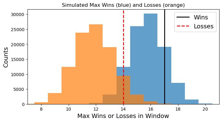
Fig 3: Max wins (blue) and losses (orange) in a 20-game window in 100,000 simulated 112 game stretches assuming a constant win probability of 0.6
So are the observed max wins/losses values consistent with a win value of \(p=0.6\)? Well, yeah, kinda. They certainly fall within the respective histograms (although the losses seem to be a bit further out on the tail than the wins). But ideally we would be able to calculate a probability for each \(p\). So let’s do that!
Let’s focus on what we set out to calculate. That is, we want to find the probability that the highest number of wins (or losses) in a 20 game window throughout the season exceeds some number \(k\). So we’ll now run our simulations for a range of \(p\) values and calculate this number by simply counting the number of max values that equal or exceed \(k\). So for wins, we will simulate our 100,000 seasons and find the most wins in a 20-game window for each. We will then count how many of these are greater than or equal to 17, and divide by the total number of simulations to get a probability. We can do the same for losses.
Figure 4 below shows these results. The blue line gives the probability that the max number of wins in a 20 game window is greater than or equal to 17 for a range of win probabilities. Likewise the orange curve shows the probability that the max number of losses is greater than or equal to 14.
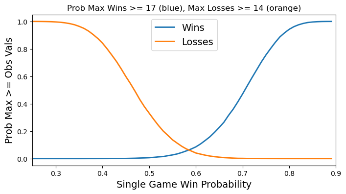
Fig 4: Probability that the max number of wins (blue) and losses (orange) exceed the observed values as a function of win probability.
These curves behave as we would expect. If the win probability is very low, then the probability of getting a max of at least 14 losses in a 20 game window is very good (i.e., 1). Likewise, if the win probability is very high, then the probability of getting a max of at least 17 wins in a 20 game window is very good (i.e., 1). However, it is odd that the intersection occurs at such a low probability (about 6%), but this could be evidence against our assumption that \(p\) is fixed for the whole season.
Figure 4 showed the individual probability curves for losses and wins as a function of individual game win probability. But we want both of these to be true at the same time (since that’s what we saw). To get the probability the max wins is greater than or equal to 17 and the max losses is greater than or equal to 14, we simply multiply the probabilities. The result is shown below in Figure 5.
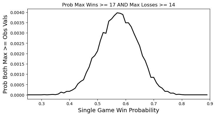
Fig 5: Product of the two probability curves from Figure 4
This curve is a little noisy, but still looks about how we would expect by multiplying the two curves in Figure 4. It has to go toward zero on the left because our blue curve goes to zero and it has to go toward zero on the right because our orange curve goes to zero. It is maximum where the two curves from Figure 4 intersect. The peak of this probability curve is around \(p=0.57\), which is very close to the cumulative winning fraction after 112 games from Figure 2. With this win probability, we would expect the team to win about 92 out of 162 games for the regular season. Not setting any records, but still pretty good.
Conclusions
By simulating the results, we were able to numerically calculate the probability of the maximum number of wins (or losses) in a 20 game window exceeding some particular value. Based on this, we see that the Phillies season probably has not been super well described by a single unchanging win probability. To properly evaluate that claim, however, we would need to do some kind of model comparison.
However, in the next part we will not be doing that! Instead we will consider a fun (?) yet highly impractical way of calculating the desired probability without simulations.
Unless otherwise noted, all the data will come from baseball-reference.com. For example, you can find the results for the Phillies season here. ↩